
Introduction to Deep Learning: How to make your




Description: Introduction to Deep Learning: How to make your own deep learning framework Ryota Tomioka (ryotomicrosoft.com) MSR Summer School 2 July 2018 Agenda This lecture covers Introduction to machine learning (keywords: model, training, inference,
Related Topics
Download Presentation
"Introduction to Deep Learning: How to make your" is the property of its rightful owner. Permission is granted to download and print the materials on this website for personal, non-commercial use only, and to display it on your personal computer provided you do not modify the materials and that you retain all copyright notices contained in the materials. By downloading content from our website, you accept the terms of this agreement.
Presentation Transcript
slide1. Introduction to Deep Learning: How to make your own deep learning framework Ryota Tomioka (ryoto@microsoft.com)
MSR Summer School
2 July 2018<br>
slide2. Agenda This lecture covers
Introduction to machine learning (keywords: model, training, inference, stochastic gradient descent, overfitting)
How to compute the gradient (keywords: backpropagation, multi-layer perceptrons, activation function)<br>
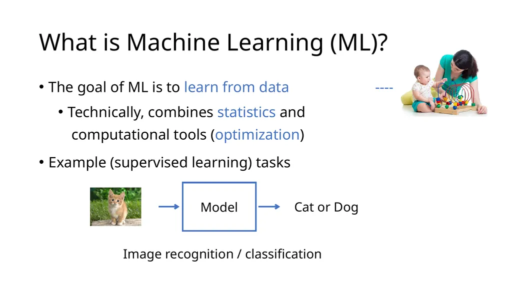
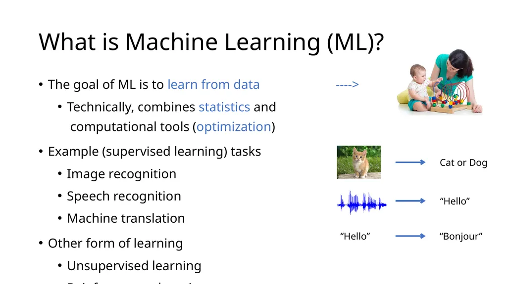
slide3. What is Machine Learning (ML)? The goal of ML is to learn from data ---->
Technically, combines statistics and computational tools (optimization)
Example (supervised learning) tasks Cat or Dog Image recognition / classification Model<br>
slide4. What is Machine Learning (ML)? The goal of ML is to learn from data ---->
Technically, combines statistics and computational tools (optimization)
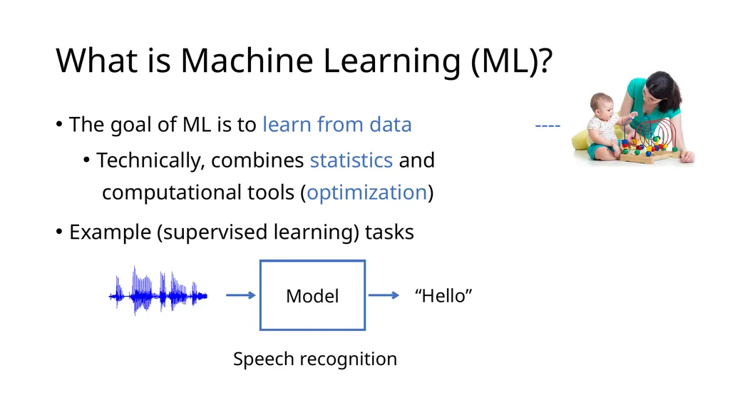
Example (supervised learning) tasks “Hello” Speech recognition Model<br>
slide5. What is Machine Learning (ML)? The goal of ML is to learn from data ---->
Technically, combines statistics and computational tools (optimization)
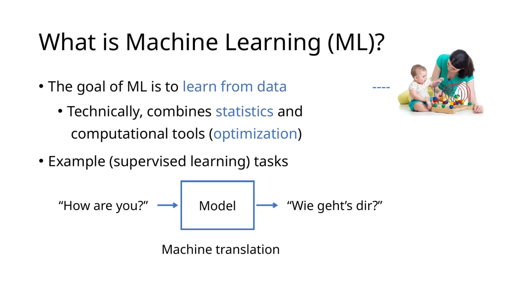
Example (supervised learning) tasks “How are you?” “Wie geht’s dir?” Machine translation Model<br>
slide6. What is Machine Learning (ML)? The goal of ML is to learn from data ---->
Technically, combines statistics and computational tools (optimization)
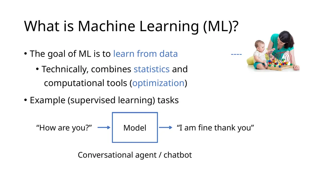
Example (supervised learning) tasks “How are you?” “I am fine thank you” Conversational agent / chatbot Model<br>
slide7. What is Machine Learning (ML)? The goal of ML is to learn from data ---->
Technically, combines statistics and computational tools (optimization)
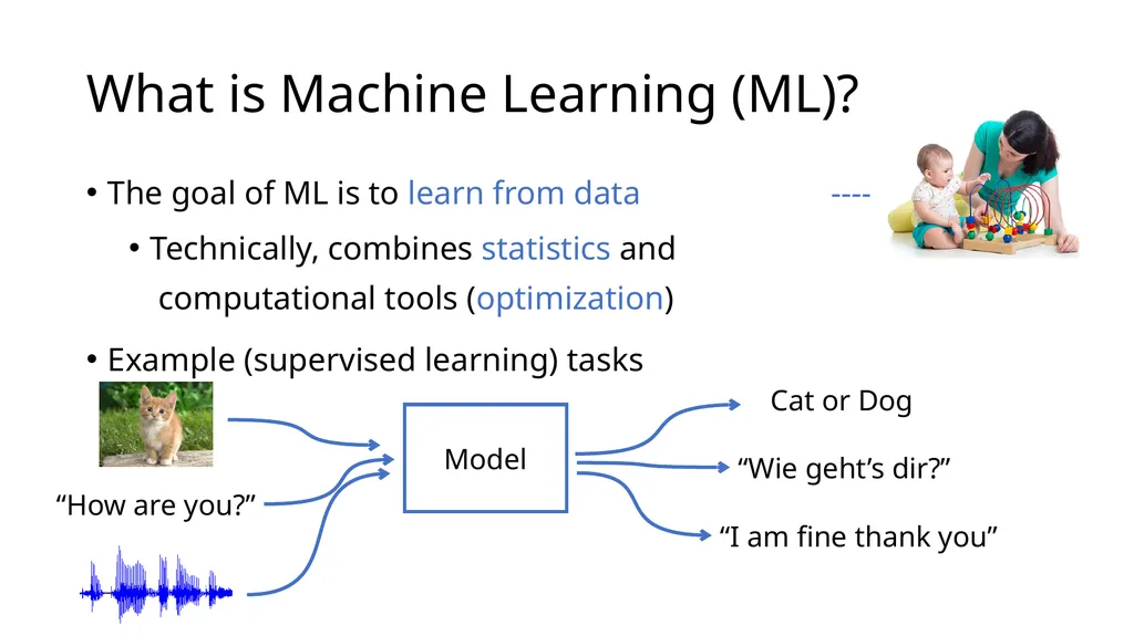
Example (supervised learning) tasks Model “How are you?” “I am fine thank you” Cat or Dog “Wie geht’s dir?”<br>
slide8. What is Machine Learning (ML)? The goal of ML is to learn from data ---->
Technically, combines statistics and computational tools (optimization)
Example (supervised learning) tasks
Image recognition
Speech recognition
Machine translation
Other form of learning
Unsupervised learning
Reinforcement learning Cat or Dog “Hello” “Hello” “Bonjour”<br>
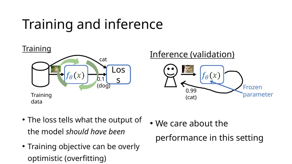
slide9. Training and inference Training
The loss tells what the output of the model should have been
Training objective can be overly optimistic (overfitting) Inference (validation)
We care about the performance in this setting Training data Loss cat 0.99
(cat) 0.1
(dog)<br>
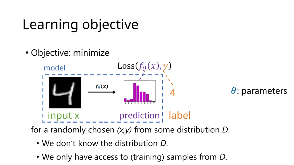
slide11. Learning objective input x label 4 prediction model<br>
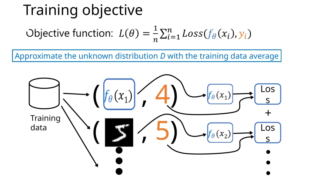
slide12. Training objective Approximate the unknown distribution D with the training data average<br>
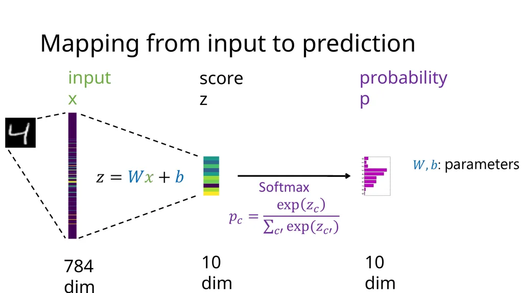
slide13. Mapping from input to prediction input x 784 dim score z 10 dim probability p 10 dim<br>
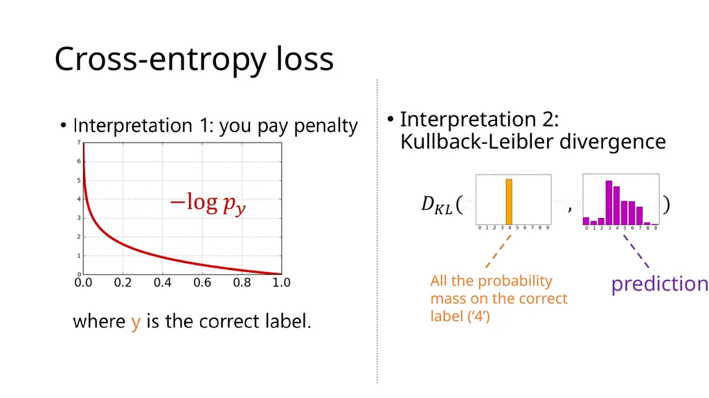
slide14. Cross-entropy loss Interpretation 2: Kullback-Leibler divergence All the probability mass on the correct label (‘4’) prediction<br>
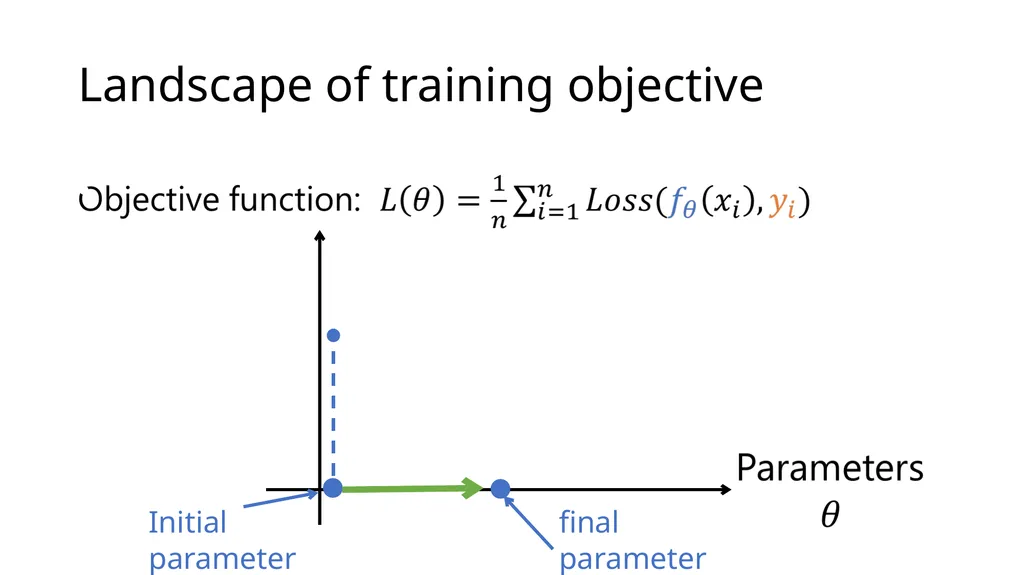
slide15. Landscape of training objective Initial parameters final parameters<br>
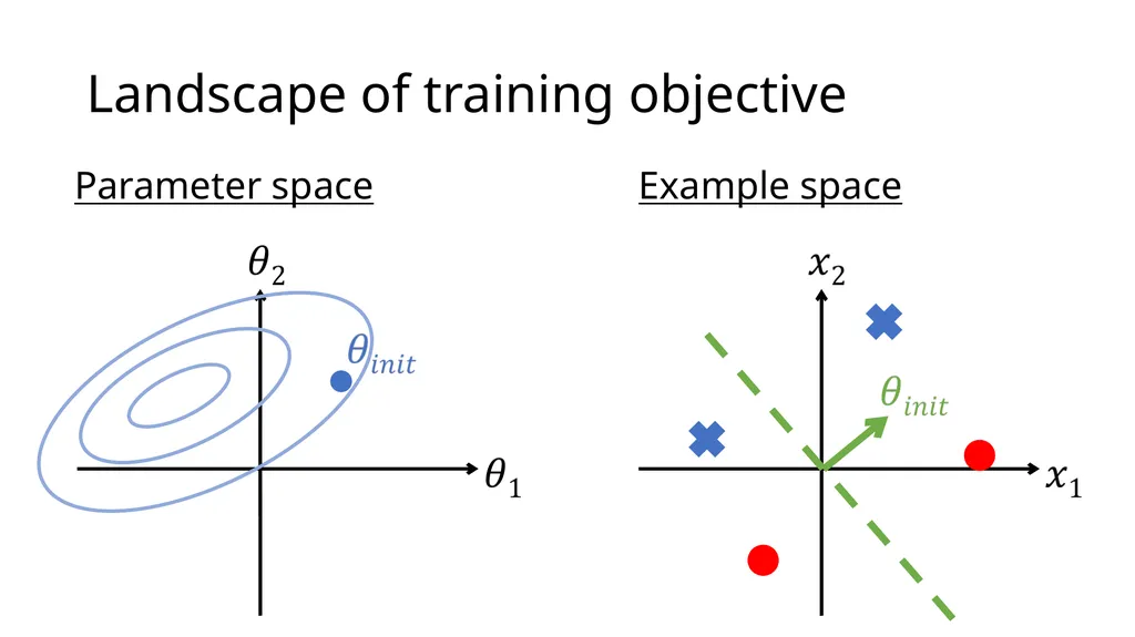
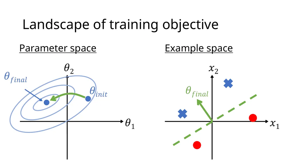
slide16. Landscape of training objective Parameter space Example space<br>
slide17. Landscape of training objective Parameter space Example space<br>
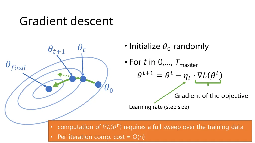
slide18. Gradient descent Gradient of the objective Learning rate (step size)<br>
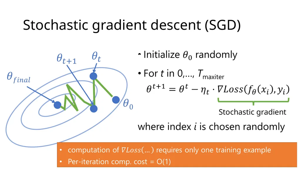
slide19. Stochastic gradient descent (SGD) Stochastic gradient<br>
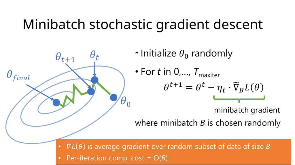
slide20. Minibatch stochastic gradient descent minibatch gradient<br>
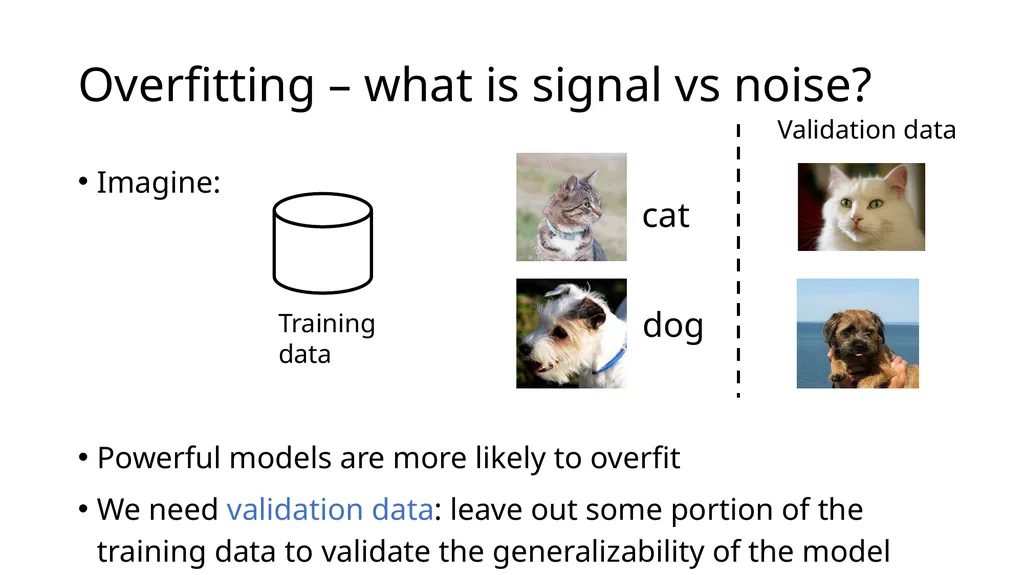
slide21. Overfitting – what is signal vs noise? Imagine:
Powerful models are more likely to overfit
We need validation data: leave out some portion of the training data to validate the generalizability of the model Training data cat dog<br>
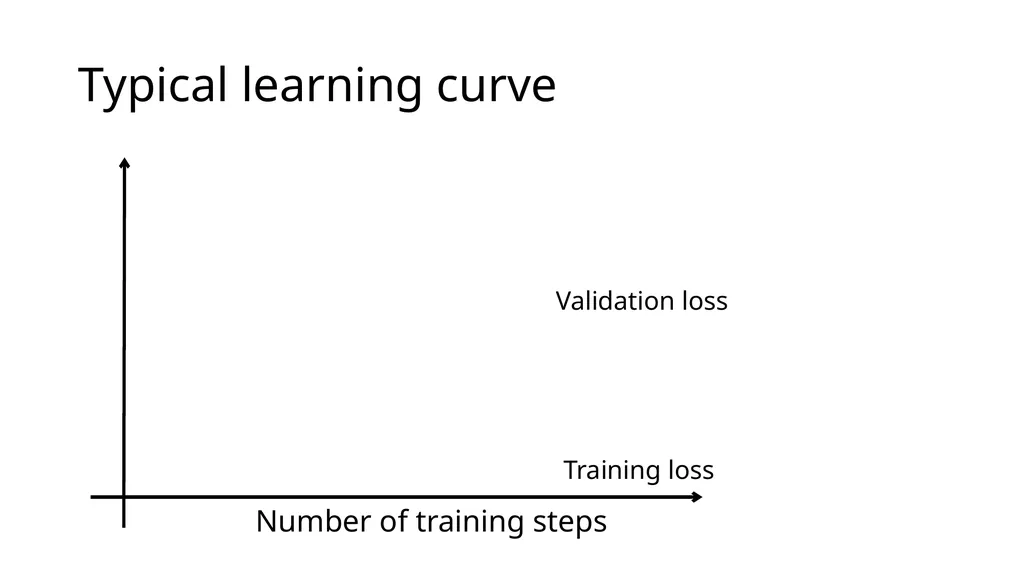
slide22. Typical learning curve Number of training steps Training loss Validation loss<br>
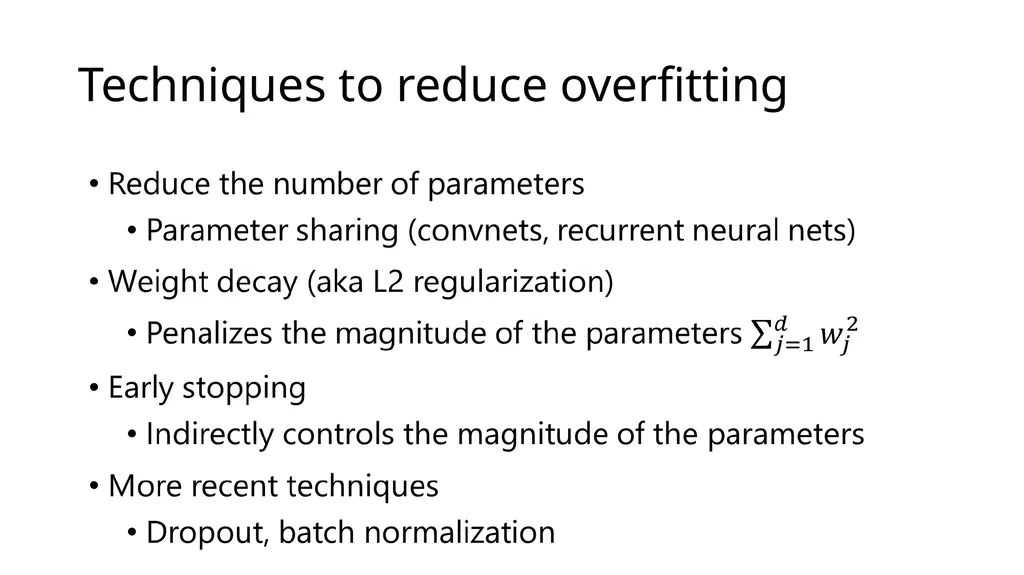
slide23. Techniques to reduce overfitting<br>
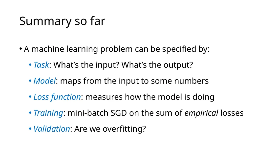
slide24. Summary so far A machine learning problem can be specified by:
Task: What’s the input? What’s the output?
Model: maps from the input to some numbers
Loss function: measures how the model is doing
Training: mini-batch SGD on the sum of empirical losses
Validation: Are we overfitting?<br>
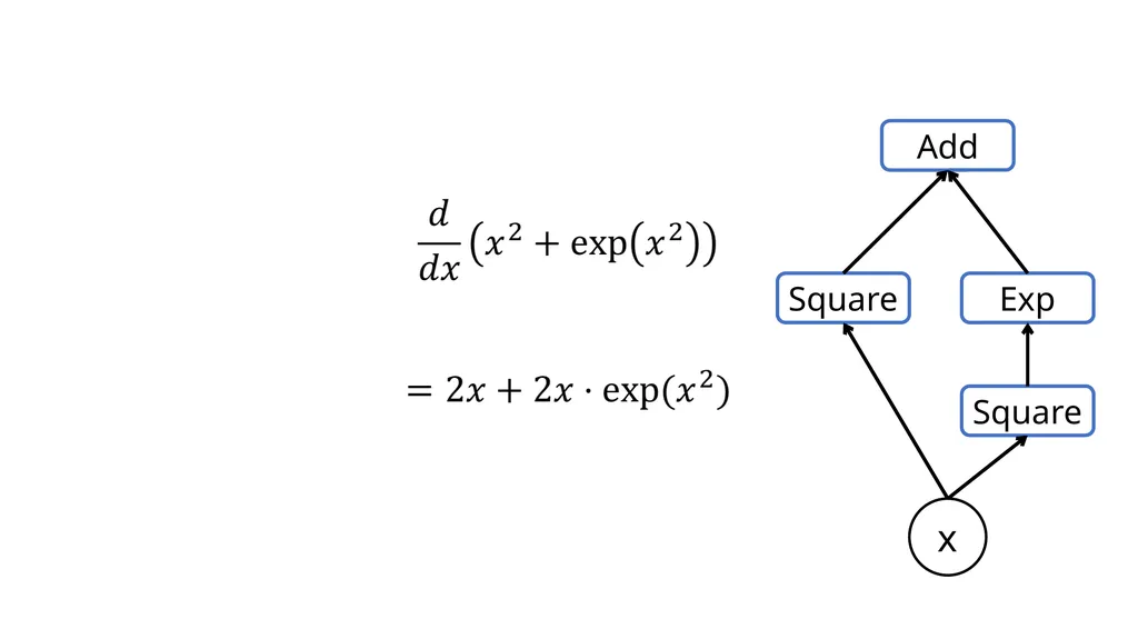
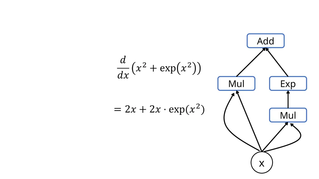
slide25. How do we compute the gradient?<br>
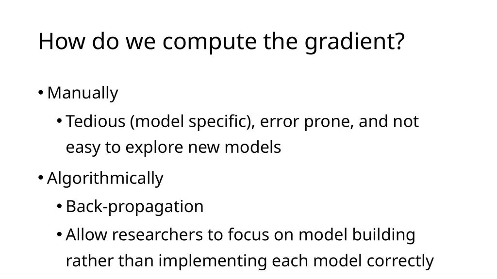
slide28. How do we compute the gradient? Manually
Tedious (model specific), error prone, and not easy to explore new models
Algorithmically
Back-propagation
Allow researchers to focus on model building rather than implementing each model correctly<br>
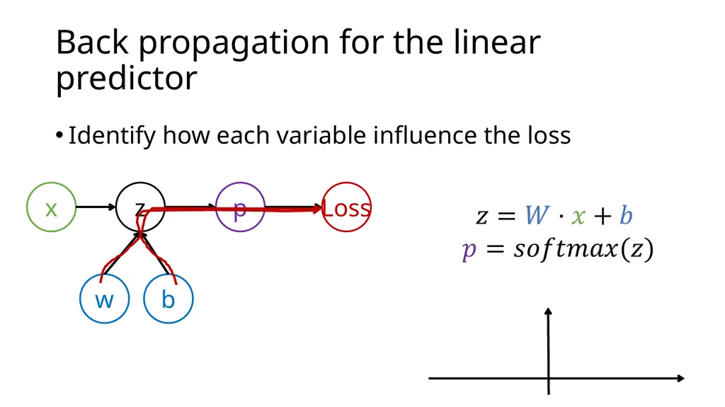
slide29. Back propagation for the linear predictor Identify how each variable influence the loss x w b z p Loss<br>
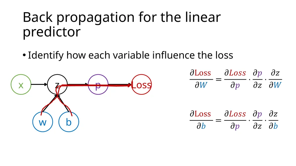
slide30. Back propagation for the linear predictor Identify how each variable influence the loss x w b z p Loss<br>
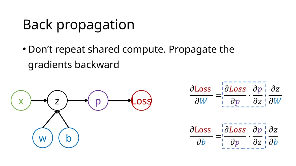
slide31. Back propagation Don’t repeat shared compute. Propagate the gradients backward x w b z p Loss<br>
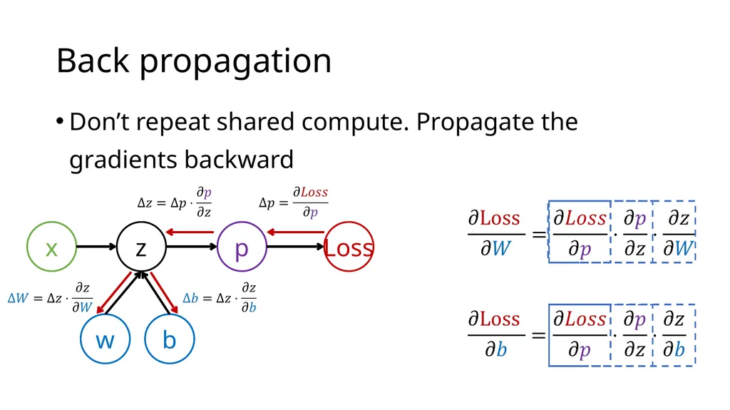
slide32. Back propagation Don’t repeat shared compute. Propagate the gradients backward x w b z p Loss<br>
slide33. Going deeper<br>
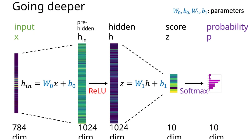
slide34. Going deeper input x 784 dim score z 1024 dim probability p Softmax 10 dim ReLU hidden h pre-
hidden hin 10 dim 1024 dim input x 784 dim score z 1024 dim probability p Softmax 10 dim ReLU hidden h pre-
hidden hin 10 dim 1024 dim<br>
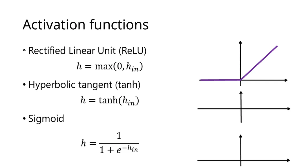
slide35. Activation functions<br>
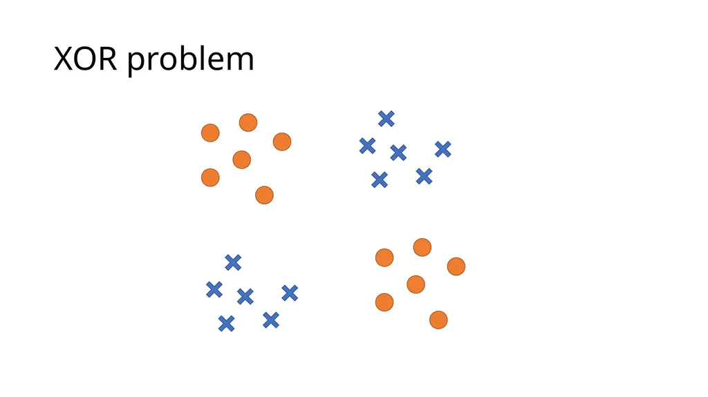
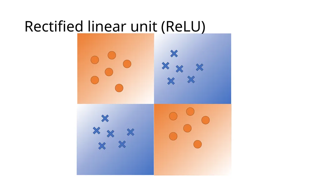
slide36. XOR problem<br>
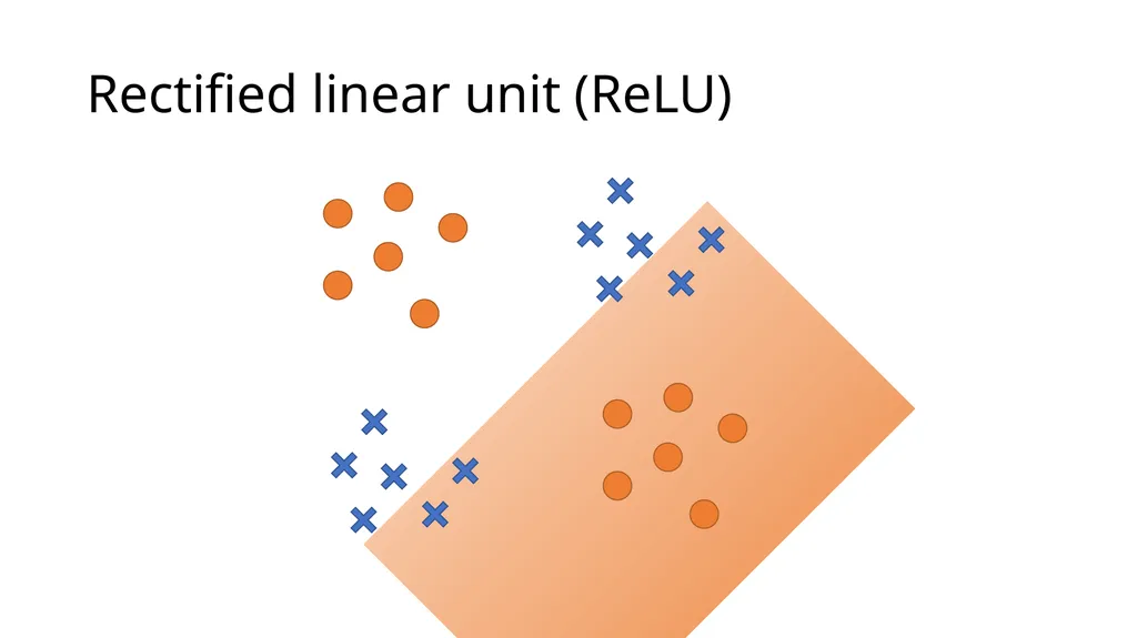
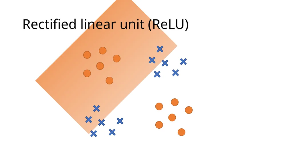
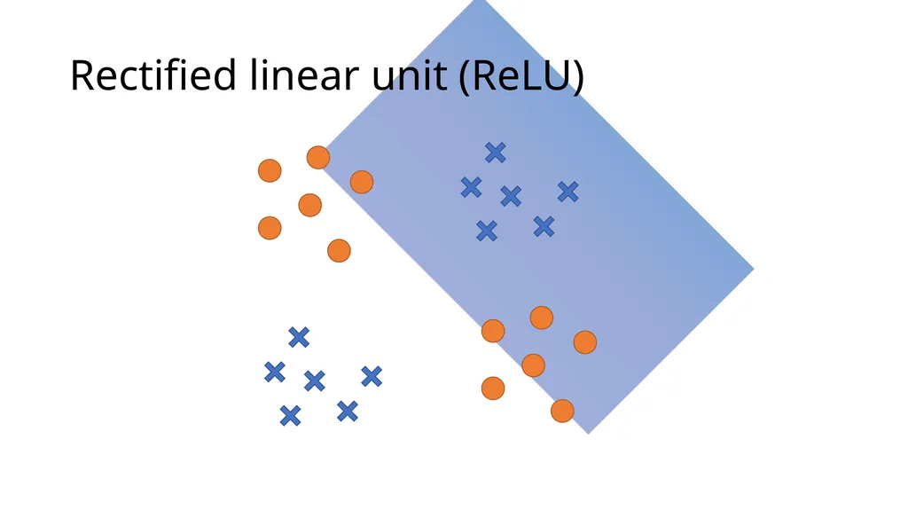
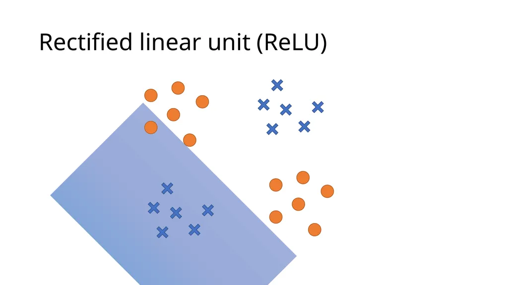
slide37. Rectified linear unit (ReLU)<br>
slide38. Rectified linear unit (ReLU)<br>
slide39. Rectified linear unit (ReLU)<br>
slide40. Rectified linear unit (ReLU)<br>
slide41. Rectified linear unit (ReLU)<br>
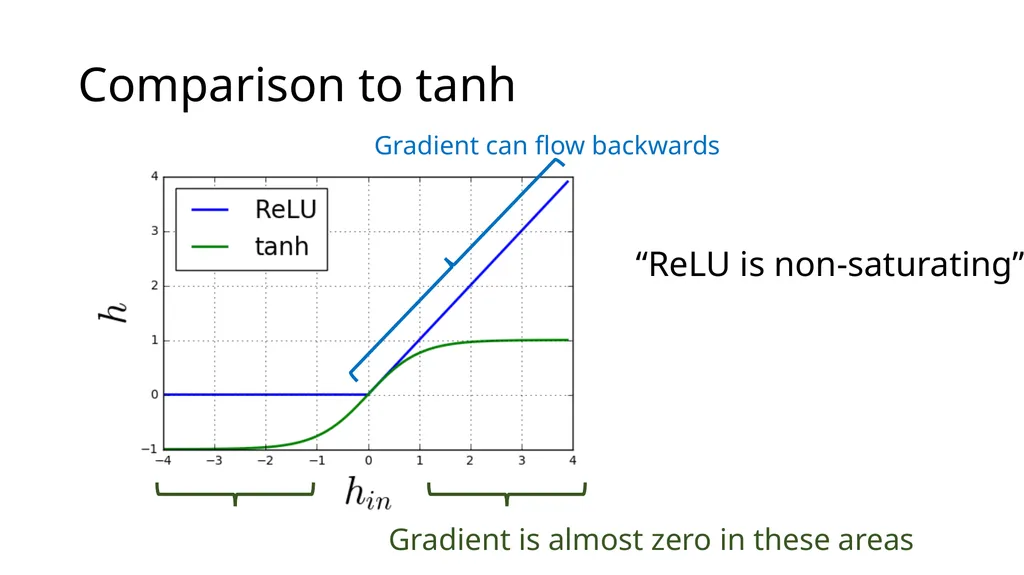
slide42. Comparison to tanh Gradient can flow backwards “ReLU is non-saturating”<br>
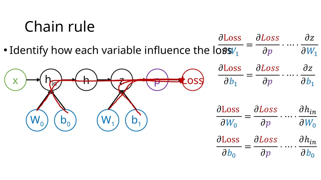
slide43. Chain rule x W0 b0 hin p Loss W1 b1 z h Identify how each variable influence the loss<br>
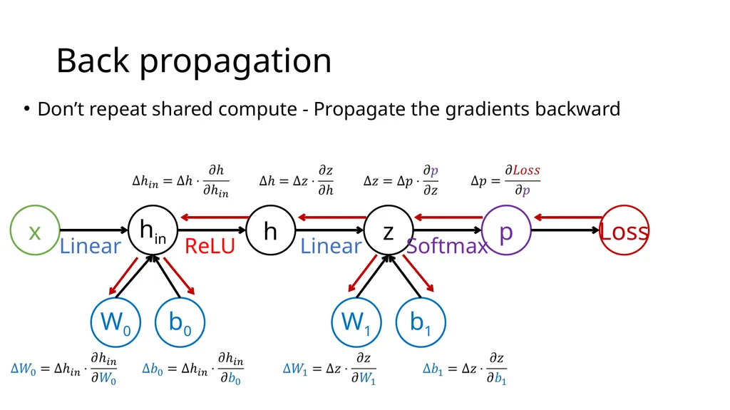
slide44. Back propagation x W0 b0 hin p Loss W1 b1 z h Softmax ReLU Linear Linear Don’t repeat shared compute - Propagate the gradients backward<br>
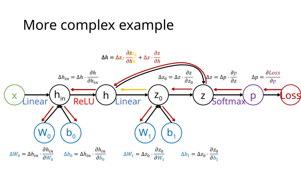
slide45. More complex example x W0 b0 hin p Loss W1 b1 z0 h Softmax ReLU Linear Linear z<br>
slide46. Demo<br>
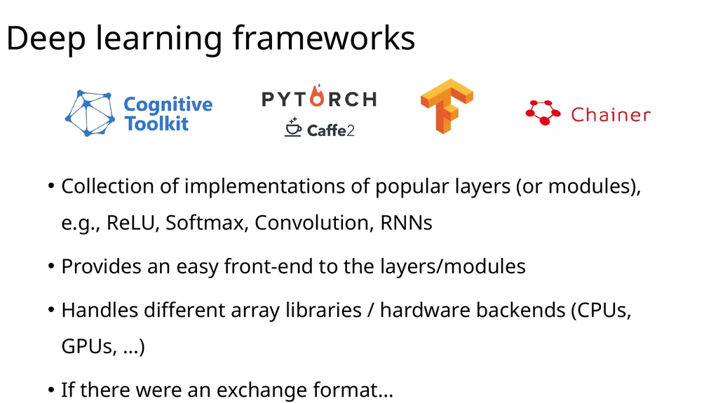
slide47. Deep learning frameworks Collection of implementations of popular layers (or modules), e.g., ReLU, Softmax, Convolution, RNNs
Provides an easy front-end to the layers/modules
Handles different array libraries / hardware backends (CPUs, GPUs, …)
If there were an exchange format…<br>
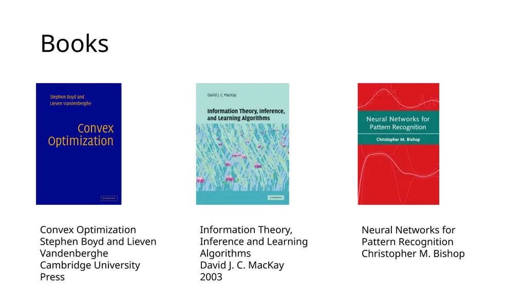
slide49. Books Convex Optimization
Stephen Boyd and Lieven Vandenberghe
Cambridge University Press Information Theory, Inference and Learning Algorithms
David J. C. MacKay
2003 Neural Networks for Pattern Recognition
Christopher M. Bishop<br>
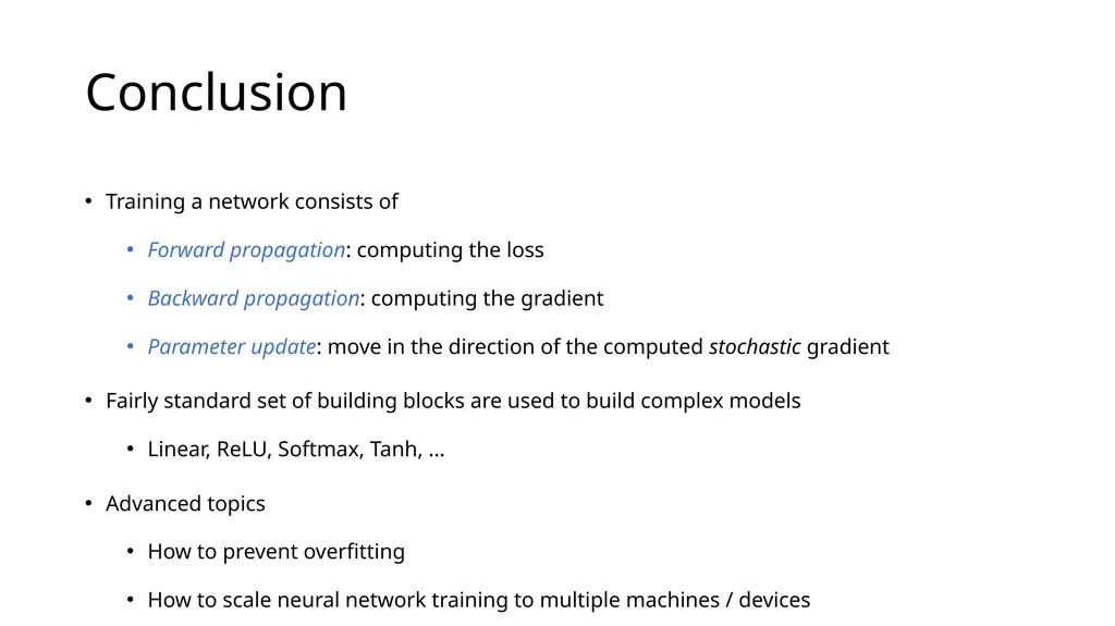
slide50. Conclusion Training a network consists of
Forward propagation: computing the loss
Backward propagation: computing the gradient
Parameter update: move in the direction of the computed stochastic gradient
Fairly standard set of building blocks are used to build complex models
Linear, ReLU, Softmax, Tanh, …
Advanced topics
How to prevent overfitting
How to scale neural network training to multiple machines / devices<br>
slide51. Advanced topics<br>
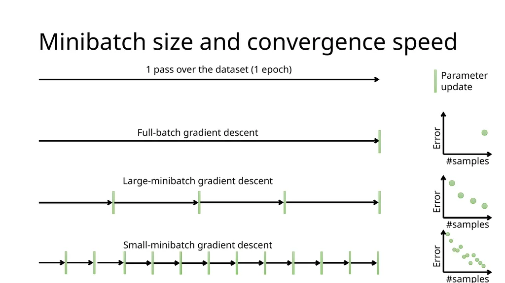
slide52. Minibatch size and convergence speed 1 pass over the dataset (1 epoch)<br>
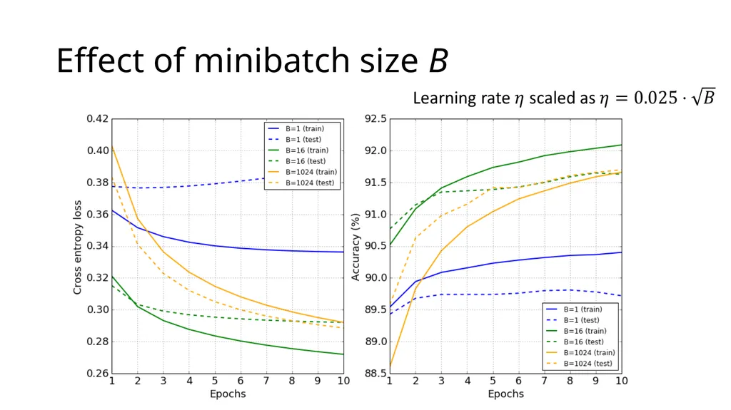
slide53. Effect of minibatch size B<br>
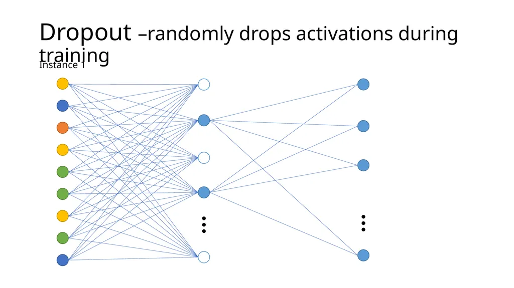
slide54. Dropout –randomly drops activations during training Instance 1<br>
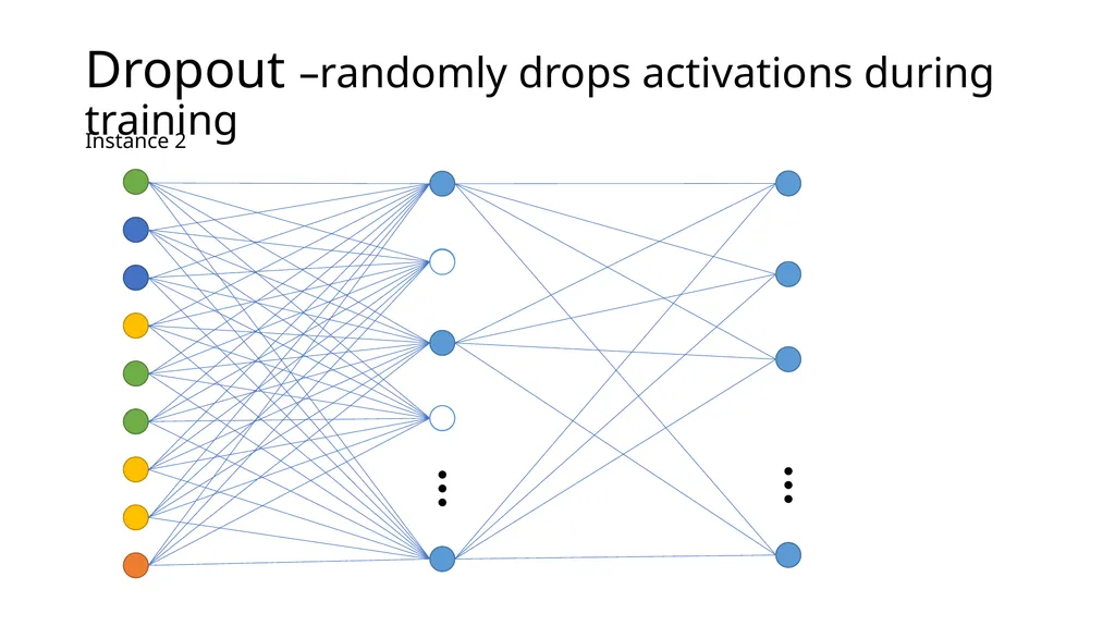
slide55. Dropout –randomly drops activations during training Instance 2<br>
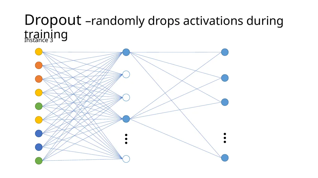
slide56. Dropout –randomly drops activations during training Instance 3<br>
slide57. Dropout Idea: randomly drop activations during training
Benefit: reduces overfitting and improves generalization
Can be implemented as a layer<br>
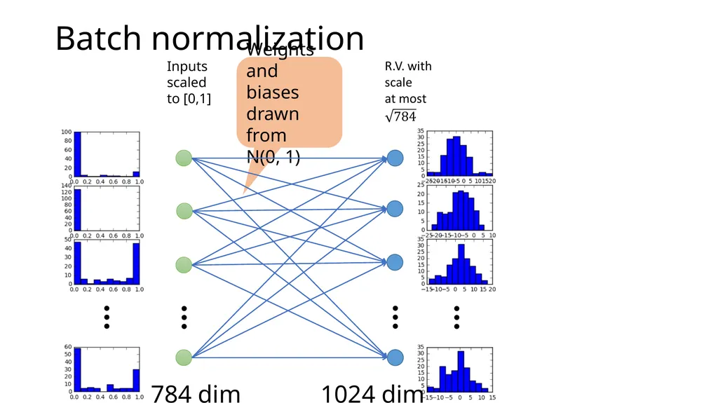
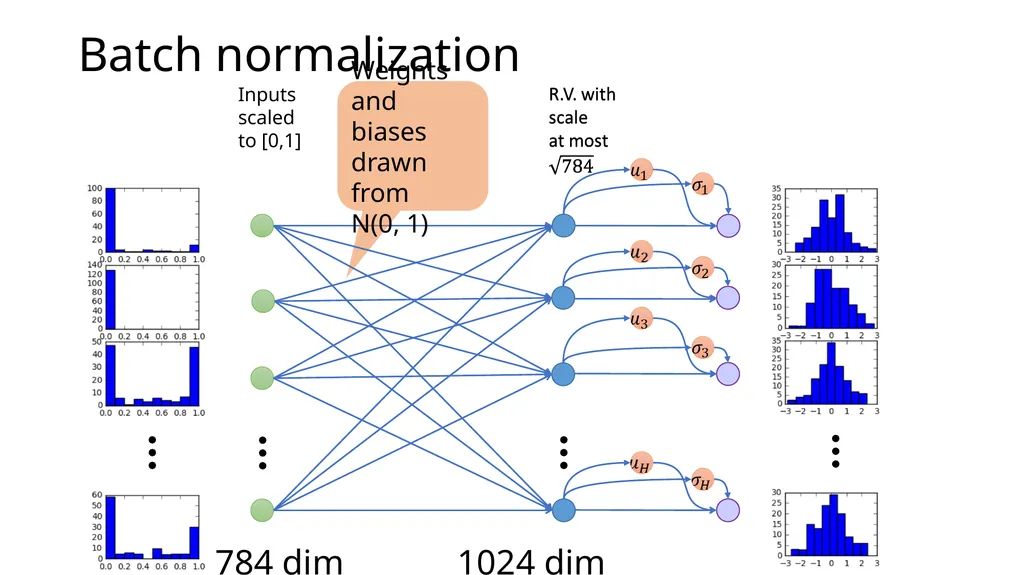
slide58. Batch normalization Inputs scaled to [0,1] 784 dim Weights and biases
drawn from
N(0, 1) 1024 dim<br>
slide59. Batch normalization 784 dim Weights and biases
drawn from
N(0, 1) 1024 dim Inputs scaled to [0,1]<br>
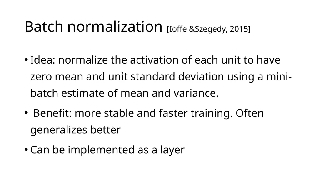
slide60. Batch normalization [Ioffe &Szegedy, 2015] Idea: normalize the activation of each unit to have zero mean and unit standard deviation using a mini-batch estimate of mean and variance.
Benefit: more stable and faster training. Often generalizes better
Can be implemented as a layer<br>
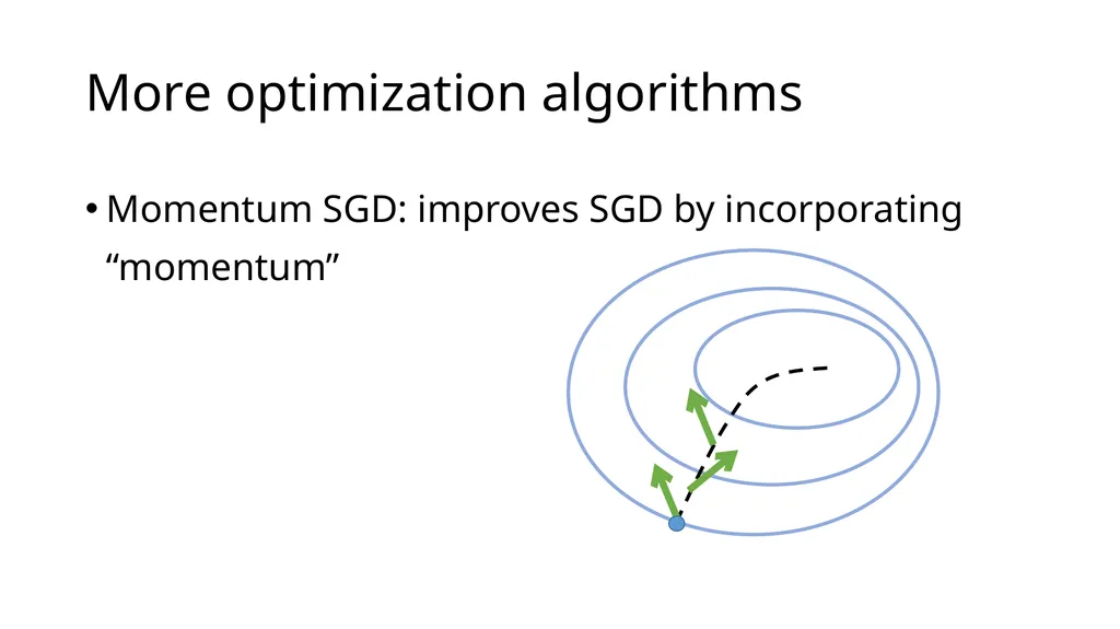
slide61. More optimization algorithms Momentum SGD: improves SGD by incorporating “momentum”<br>
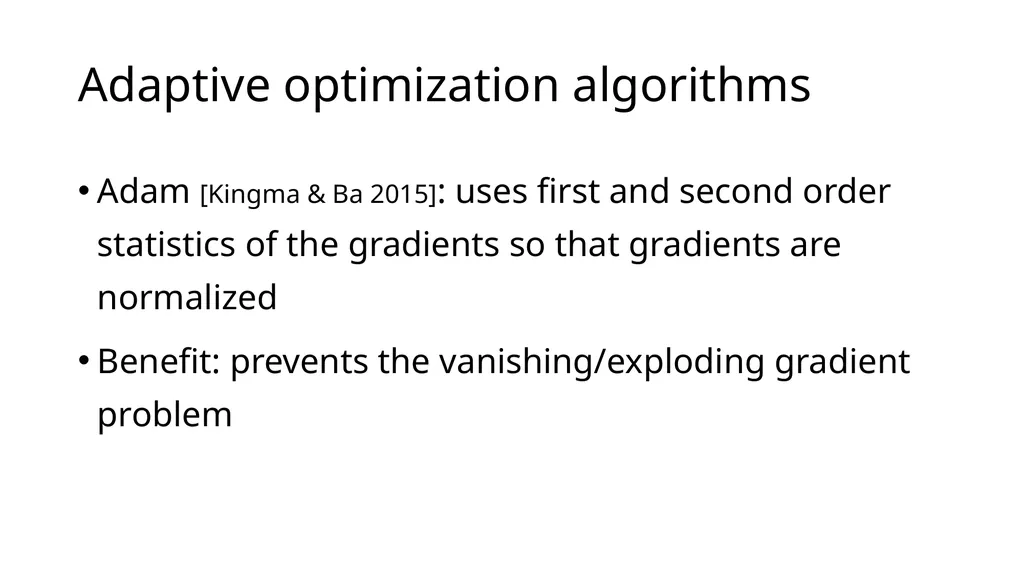
slide62. Adaptive optimization algorithms Adam [Kingma & Ba 2015]: uses first and second order statistics of the gradients so that gradients are normalized
Benefit: prevents the vanishing/exploding gradient problem<br>
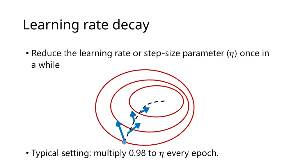
slide63. Learning rate decay<br>
slide64. Summary Training and inference
Training objective and optimization
Neural networks and backpropagation
Importance of software tools – turns research into Lego block engineering
Various tricks to speed-up training and reduce overfitting<br>
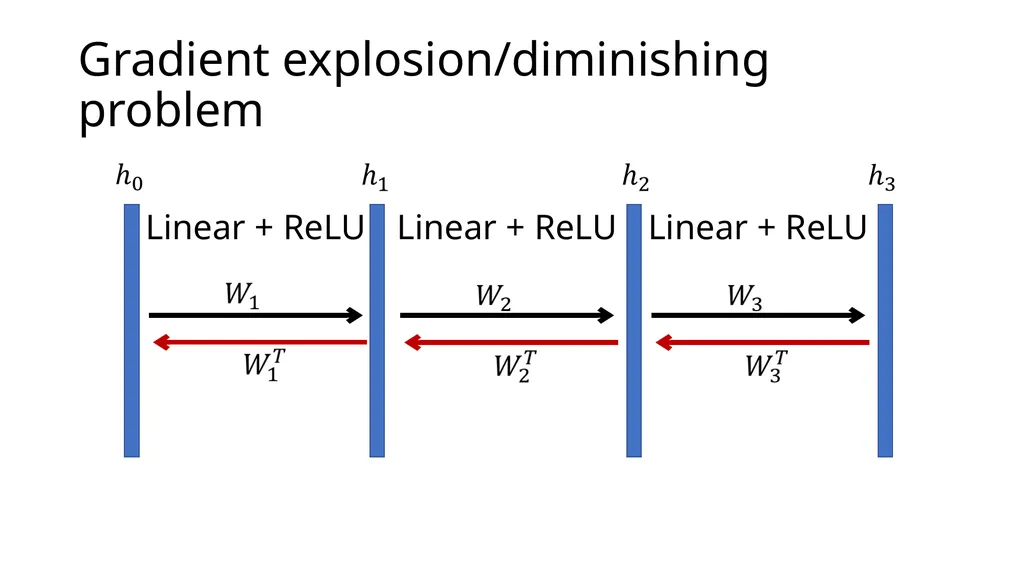
slide65. Gradient explosion/diminishing problem Linear + ReLU Linear + ReLU Linear + ReLU<br>
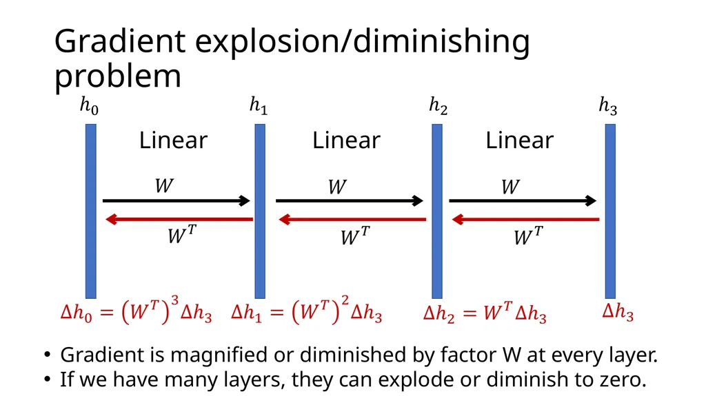
slide66. Gradient explosion/diminishing problem Linear Linear Linear Gradient is magnified or diminished by factor W at every layer.
If we have many layers, they can explode or diminish to zero.<br>
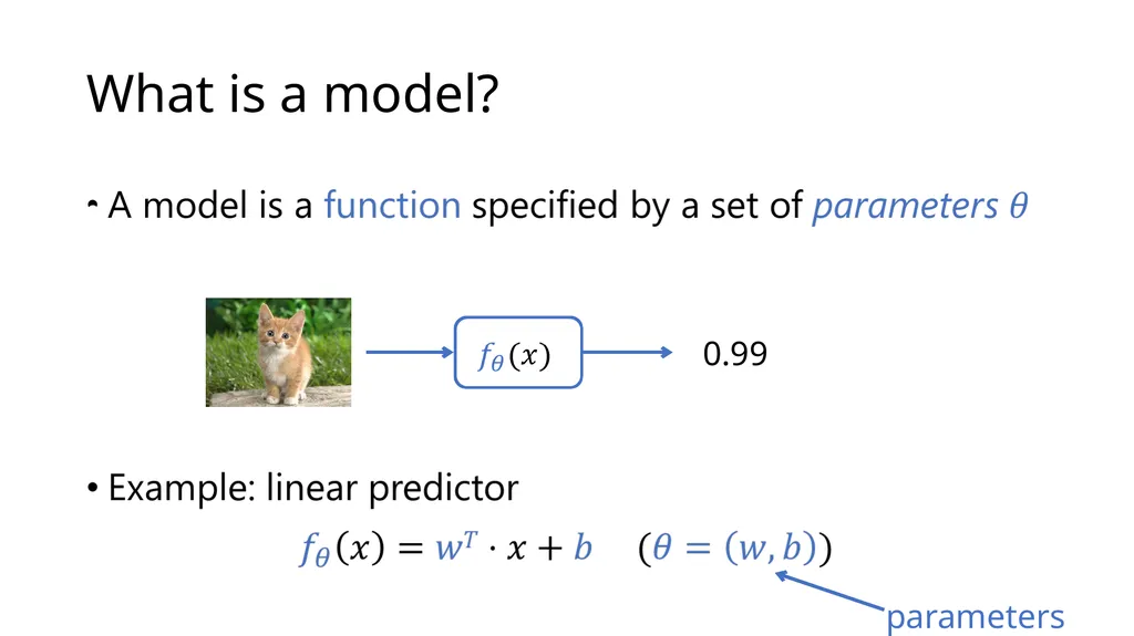
slide67. What is a model? 0.99 parameters<br>
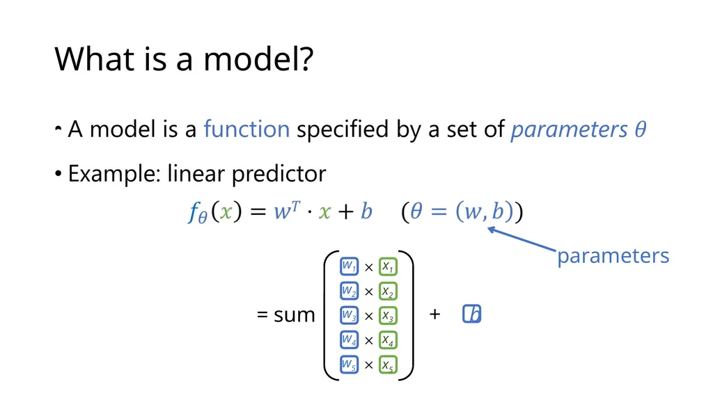
slide68. What is a model? parameters = sum + b w1 w2 w3 w4 w5 x1 x2 x3 x4 x5<br>
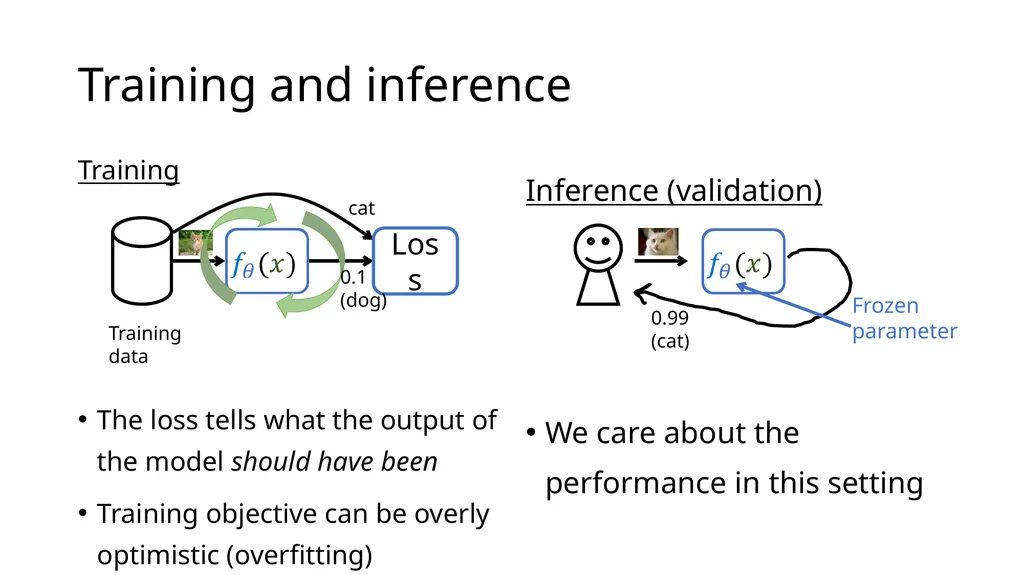
slide69. Training and inference Training
The loss tells what the output of the model should have been
Training objective can be overly optimistic (overfitting) Inference (validation)
We care about the performance in this setting Training data Loss cat 0.99
(cat) 0.1
(dog)<br>
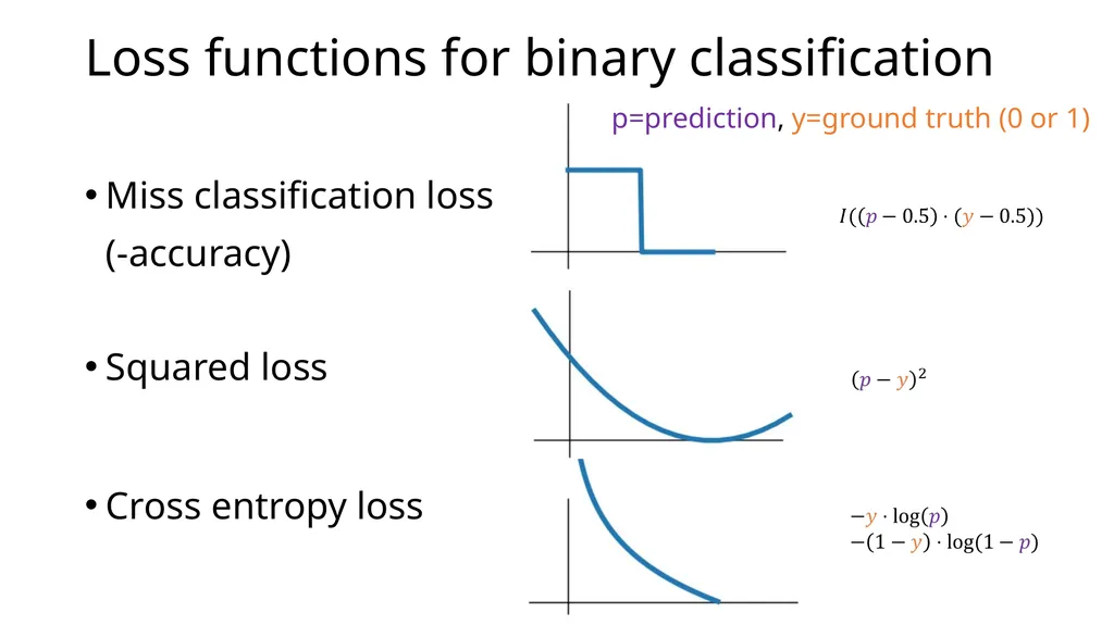
slide71. Loss functions for binary classification Miss classification loss (-accuracy)
Squared loss
Cross entropy loss p=prediction, y=ground truth (0 or 1)<br>
MSR Summer School
2 July 2018<br>
slide2. Agenda This lecture covers
Introduction to machine learning (keywords: model, training, inference, stochastic gradient descent, overfitting)
How to compute the gradient (keywords: backpropagation, multi-layer perceptrons, activation function)<br>
slide3. What is Machine Learning (ML)? The goal of ML is to learn from data ---->
Technically, combines statistics and computational tools (optimization)
Example (supervised learning) tasks Cat or Dog Image recognition / classification Model<br>
slide4. What is Machine Learning (ML)? The goal of ML is to learn from data ---->
Technically, combines statistics and computational tools (optimization)
Example (supervised learning) tasks “Hello” Speech recognition Model<br>
slide5. What is Machine Learning (ML)? The goal of ML is to learn from data ---->
Technically, combines statistics and computational tools (optimization)
Example (supervised learning) tasks “How are you?” “Wie geht’s dir?” Machine translation Model<br>
slide6. What is Machine Learning (ML)? The goal of ML is to learn from data ---->
Technically, combines statistics and computational tools (optimization)
Example (supervised learning) tasks “How are you?” “I am fine thank you” Conversational agent / chatbot Model<br>
slide7. What is Machine Learning (ML)? The goal of ML is to learn from data ---->
Technically, combines statistics and computational tools (optimization)
Example (supervised learning) tasks Model “How are you?” “I am fine thank you” Cat or Dog “Wie geht’s dir?”<br>
slide8. What is Machine Learning (ML)? The goal of ML is to learn from data ---->
Technically, combines statistics and computational tools (optimization)
Example (supervised learning) tasks
Image recognition
Speech recognition
Machine translation
Other form of learning
Unsupervised learning
Reinforcement learning Cat or Dog “Hello” “Hello” “Bonjour”<br>
slide9. Training and inference Training
The loss tells what the output of the model should have been
Training objective can be overly optimistic (overfitting) Inference (validation)
We care about the performance in this setting Training data Loss cat 0.99
(cat) 0.1
(dog)<br>
slide11. Learning objective input x label 4 prediction model<br>
slide12. Training objective Approximate the unknown distribution D with the training data average<br>
slide13. Mapping from input to prediction input x 784 dim score z 10 dim probability p 10 dim<br>
slide14. Cross-entropy loss Interpretation 2: Kullback-Leibler divergence All the probability mass on the correct label (‘4’) prediction<br>
slide15. Landscape of training objective Initial parameters final parameters<br>
slide16. Landscape of training objective Parameter space Example space<br>
slide17. Landscape of training objective Parameter space Example space<br>
slide18. Gradient descent Gradient of the objective Learning rate (step size)<br>
slide19. Stochastic gradient descent (SGD) Stochastic gradient<br>
slide20. Minibatch stochastic gradient descent minibatch gradient<br>
slide21. Overfitting – what is signal vs noise? Imagine:
Powerful models are more likely to overfit
We need validation data: leave out some portion of the training data to validate the generalizability of the model Training data cat dog<br>
slide22. Typical learning curve Number of training steps Training loss Validation loss<br>
slide23. Techniques to reduce overfitting<br>
slide24. Summary so far A machine learning problem can be specified by:
Task: What’s the input? What’s the output?
Model: maps from the input to some numbers
Loss function: measures how the model is doing
Training: mini-batch SGD on the sum of empirical losses
Validation: Are we overfitting?<br>
slide25. How do we compute the gradient?<br>
slide28. How do we compute the gradient? Manually
Tedious (model specific), error prone, and not easy to explore new models
Algorithmically
Back-propagation
Allow researchers to focus on model building rather than implementing each model correctly<br>
slide29. Back propagation for the linear predictor Identify how each variable influence the loss x w b z p Loss<br>
slide30. Back propagation for the linear predictor Identify how each variable influence the loss x w b z p Loss<br>
slide31. Back propagation Don’t repeat shared compute. Propagate the gradients backward x w b z p Loss<br>
slide32. Back propagation Don’t repeat shared compute. Propagate the gradients backward x w b z p Loss<br>
slide33. Going deeper<br>
slide34. Going deeper input x 784 dim score z 1024 dim probability p Softmax 10 dim ReLU hidden h pre-
hidden hin 10 dim 1024 dim input x 784 dim score z 1024 dim probability p Softmax 10 dim ReLU hidden h pre-
hidden hin 10 dim 1024 dim<br>
slide35. Activation functions<br>
slide36. XOR problem<br>
slide37. Rectified linear unit (ReLU)<br>
slide38. Rectified linear unit (ReLU)<br>
slide39. Rectified linear unit (ReLU)<br>
slide40. Rectified linear unit (ReLU)<br>
slide41. Rectified linear unit (ReLU)<br>
slide42. Comparison to tanh Gradient can flow backwards “ReLU is non-saturating”<br>
slide43. Chain rule x W0 b0 hin p Loss W1 b1 z h Identify how each variable influence the loss<br>
slide44. Back propagation x W0 b0 hin p Loss W1 b1 z h Softmax ReLU Linear Linear Don’t repeat shared compute - Propagate the gradients backward<br>
slide45. More complex example x W0 b0 hin p Loss W1 b1 z0 h Softmax ReLU Linear Linear z<br>
slide46. Demo<br>
slide47. Deep learning frameworks Collection of implementations of popular layers (or modules), e.g., ReLU, Softmax, Convolution, RNNs
Provides an easy front-end to the layers/modules
Handles different array libraries / hardware backends (CPUs, GPUs, …)
If there were an exchange format…<br>
slide49. Books Convex Optimization
Stephen Boyd and Lieven Vandenberghe
Cambridge University Press Information Theory, Inference and Learning Algorithms
David J. C. MacKay
2003 Neural Networks for Pattern Recognition
Christopher M. Bishop<br>
slide50. Conclusion Training a network consists of
Forward propagation: computing the loss
Backward propagation: computing the gradient
Parameter update: move in the direction of the computed stochastic gradient
Fairly standard set of building blocks are used to build complex models
Linear, ReLU, Softmax, Tanh, …
Advanced topics
How to prevent overfitting
How to scale neural network training to multiple machines / devices<br>
slide51. Advanced topics<br>
slide52. Minibatch size and convergence speed 1 pass over the dataset (1 epoch)<br>
slide53. Effect of minibatch size B<br>
slide54. Dropout –randomly drops activations during training Instance 1<br>
slide55. Dropout –randomly drops activations during training Instance 2<br>
slide56. Dropout –randomly drops activations during training Instance 3<br>
slide57. Dropout Idea: randomly drop activations during training
Benefit: reduces overfitting and improves generalization
Can be implemented as a layer<br>
slide58. Batch normalization Inputs scaled to [0,1] 784 dim Weights and biases
drawn from
N(0, 1) 1024 dim<br>
slide59. Batch normalization 784 dim Weights and biases
drawn from
N(0, 1) 1024 dim Inputs scaled to [0,1]<br>
slide60. Batch normalization [Ioffe &Szegedy, 2015] Idea: normalize the activation of each unit to have zero mean and unit standard deviation using a mini-batch estimate of mean and variance.
Benefit: more stable and faster training. Often generalizes better
Can be implemented as a layer<br>
slide61. More optimization algorithms Momentum SGD: improves SGD by incorporating “momentum”<br>
slide62. Adaptive optimization algorithms Adam [Kingma & Ba 2015]: uses first and second order statistics of the gradients so that gradients are normalized
Benefit: prevents the vanishing/exploding gradient problem<br>
slide63. Learning rate decay<br>
slide64. Summary Training and inference
Training objective and optimization
Neural networks and backpropagation
Importance of software tools – turns research into Lego block engineering
Various tricks to speed-up training and reduce overfitting<br>
slide65. Gradient explosion/diminishing problem Linear + ReLU Linear + ReLU Linear + ReLU<br>
slide66. Gradient explosion/diminishing problem Linear Linear Linear Gradient is magnified or diminished by factor W at every layer.
If we have many layers, they can explode or diminish to zero.<br>
slide67. What is a model? 0.99 parameters<br>
slide68. What is a model? parameters = sum + b w1 w2 w3 w4 w5 x1 x2 x3 x4 x5<br>
slide69. Training and inference Training
The loss tells what the output of the model should have been
Training objective can be overly optimistic (overfitting) Inference (validation)
We care about the performance in this setting Training data Loss cat 0.99
(cat) 0.1
(dog)<br>
slide71. Loss functions for binary classification Miss classification loss (-accuracy)
Squared loss
Cross entropy loss p=prediction, y=ground truth (0 or 1)<br>