Introduction to R Data Analysis and Calculations

slide1. Introduction to R Data Analysis and CalculationsKatia Oleinikkoleinik@bu.eduResearch Computing ServicesBoston University http://www.bu.edu/tech/research/<br>
slide2. 2 Charlie Jahnke cjahnke@bu.edu

Katia Oleinik koleinik@bu.edu<br>
slide3. Outline Introduction
Help System
Variables
R environment
Vectors
Matrices
Datasets (data frames)
Lists
Online Resources 3<br>
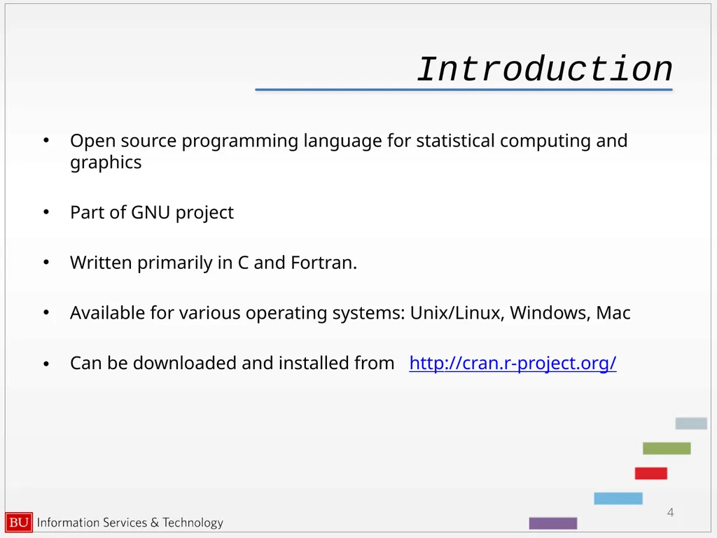
slide4. Introduction Open source programming language for statistical computing and graphics

Part of GNU project

Written primarily in C and Fortran.

Available for various operating systems: Unix/Linux, Windows, Mac

Can be downloaded and installed from http://cran.r-project.org/ 4<br>
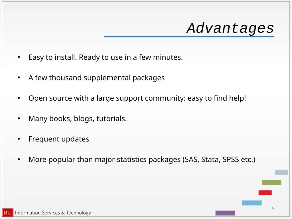
slide5. Advantages Easy to install. Ready to use in a few minutes.

A few thousand supplemental packages

Open source with a large support community: easy to find help!

Many books, blogs, tutorials.

Frequent updates

More popular than major statistics packages (SAS, Stata, SPSS etc.) 5<br>
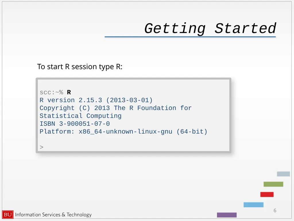
slide6. Getting Started To start R session type R: 6 scc:~% R
R version 2.15.3 (2013-03-01)
Copyright (C) 2013 The R Foundation for Statistical Computing
ISBN 3-900051-07-0
Platform: x86_64-unknown-linux-gnu (64-bit)
><br>
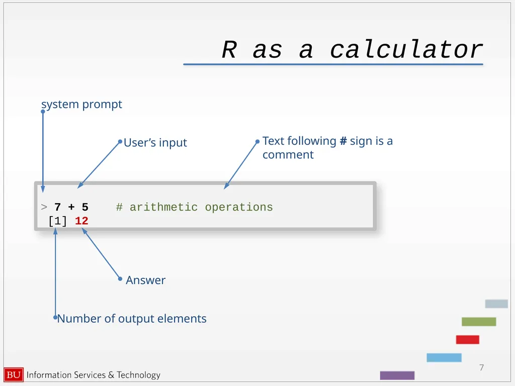
slide7. > 7 + 5 # arithmetic operations
[1] 12 R as a calculator system prompt User’s input Text following # sign is a comment Number of output elements Answer 7<br>
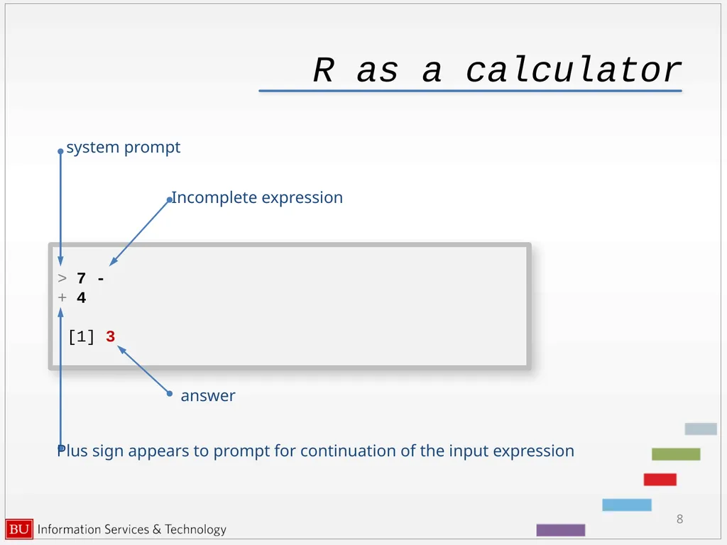
slide8. > 7 -
+ 4

[1] 3 R as a calculator system prompt Incomplete expression Plus sign appears to prompt for continuation of the input expression answer 8<br>
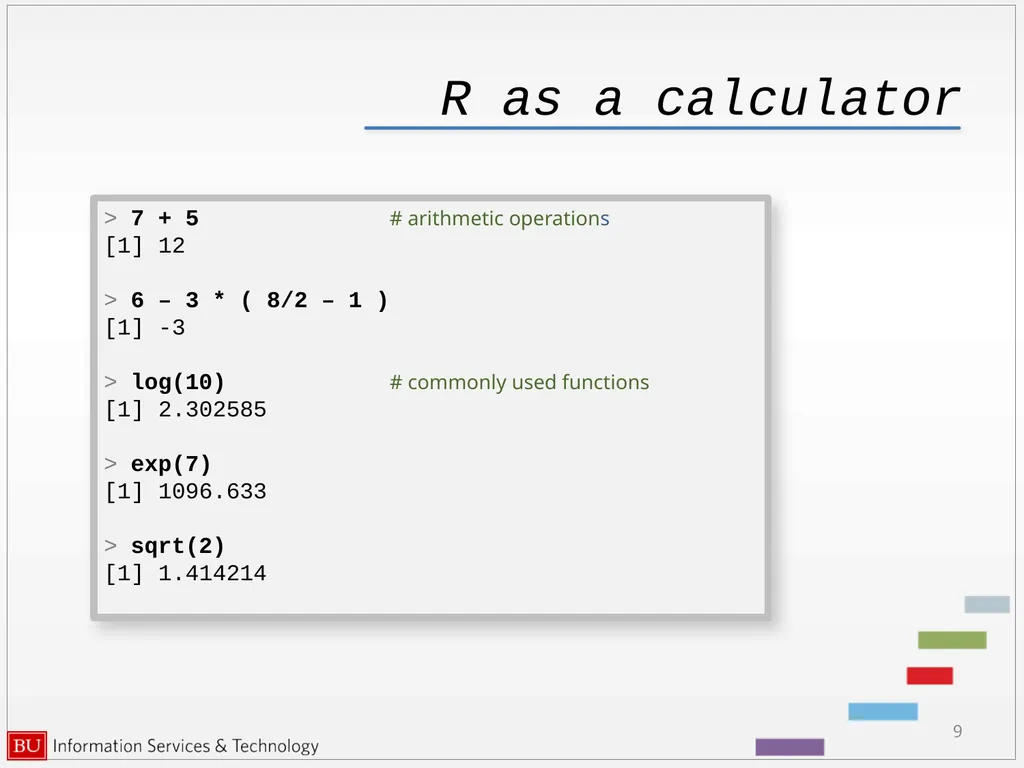
slide9. R as a calculator 9 > 7 + 5 # arithmetic operations
[1] 12

> 6 – 3 * ( 8/2 – 1 )
[1] -3

> log(10) # commonly used functions
[1] 2.302585

> exp(7)
[1] 1096.633

> sqrt(2)
[1] 1.414214<br>
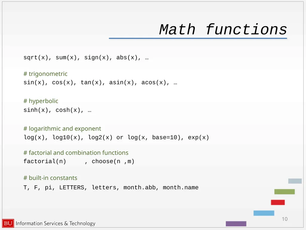
slide10. Math functions sqrt(x), sum(x), sign(x), abs(x), …

# trigonometric
sin(x), cos(x), tan(x), asin(x), acos(x), …

# hyperbolic
sinh(x), cosh(x), …

# logarithmic and exponent
log(x), log10(x), log2(x) or log(x, base=10), exp(x)
# factorial and combination functions
factorial(n) , choose(n ,m)

# built-in constants
T, F, pi, LETTERS, letters, month.abb, month.name 10<br>
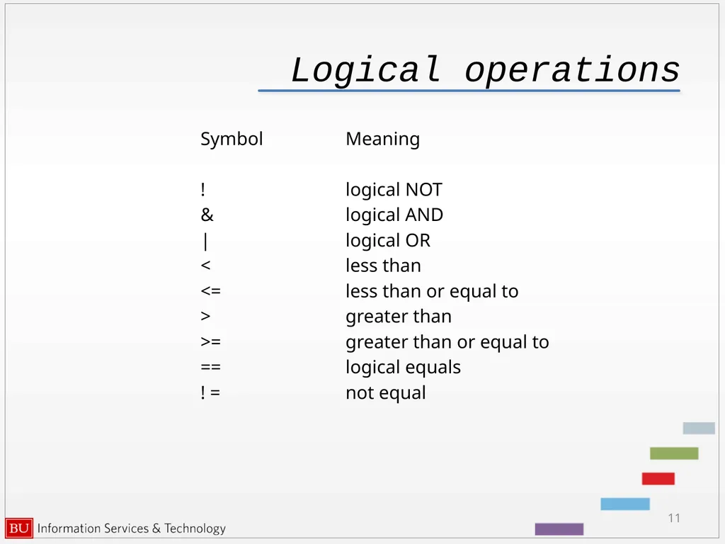
slide11. Logical operations Symbol Meaning

! logical NOT
& logical AND
| logical OR
< less than
<= less than or equal to
> greater than
>= greater than or equal to
== logical equals
! = not equal 11<br>
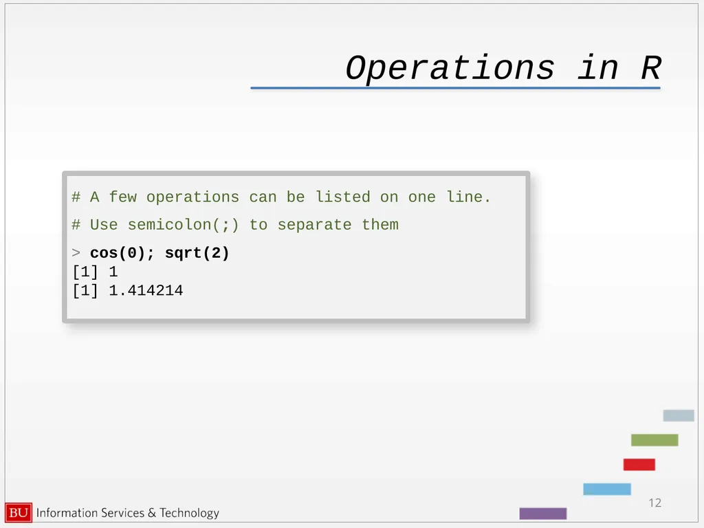
slide12. Operations in R 12 # A few operations can be listed on one line.
# Use semicolon(;) to separate them
> cos(0); sqrt(2)
[1] 1
[1] 1.414214<br>
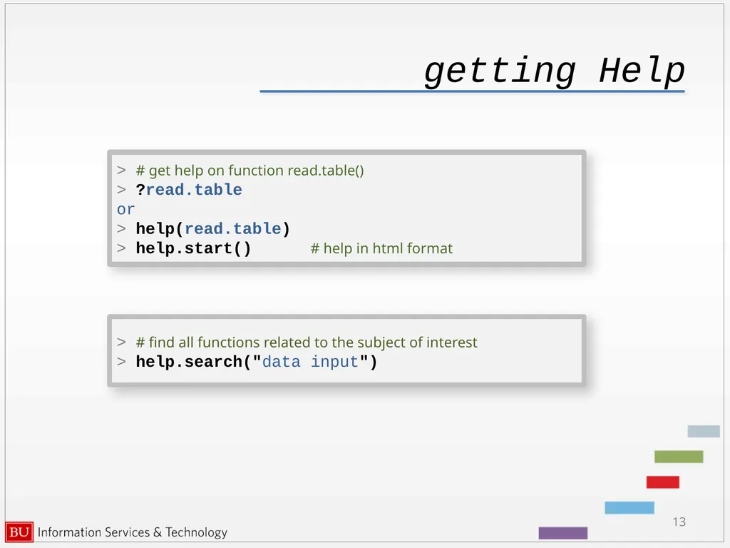
slide13. getting Help 13 > # get help on function read.table()
> ?read.table
or
> help(read.table)
> help.start() # help in html format > # find all functions related to the subject of interest
> help.search("data input")<br>
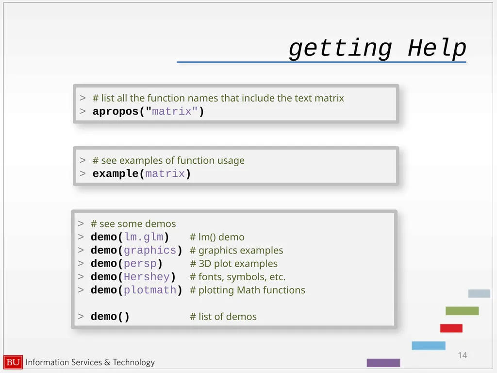
slide14. getting Help 14 > # list all the function names that include the text matrix
> apropos("matrix") > # see examples of function usage
> example(matrix) > # see some demos
> demo(lm.glm) # lm() demo
> demo(graphics) # graphics examples
> demo(persp) # 3D plot examples
> demo(Hershey) # fonts, symbols, etc.
> demo(plotmath) # plotting Math functions

> demo() # list of demos<br>
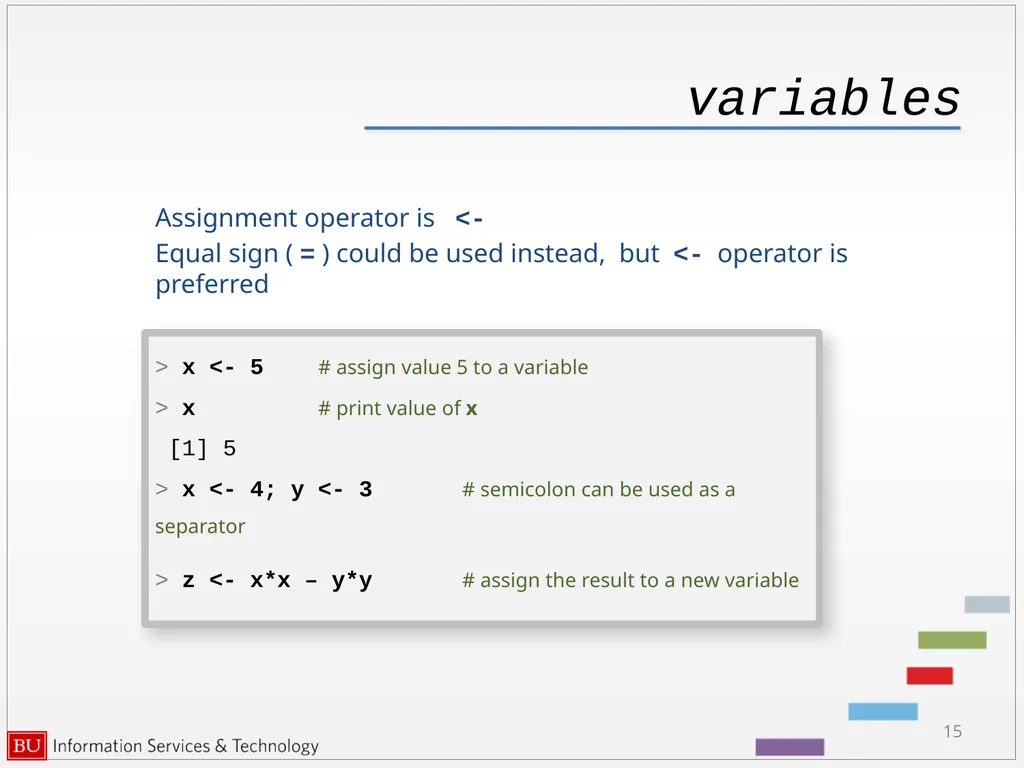
slide15. variables Assignment operator is <-
Equal sign ( = ) could be used instead, but <- operator is preferred 15 > x <- 5 # assign value 5 to a variable
> x # print value of x
[1] 5
> x <- 4; y <- 3 # semicolon can be used as a separator

> z <- x*x – y*y # assign the result to a new variable<br>
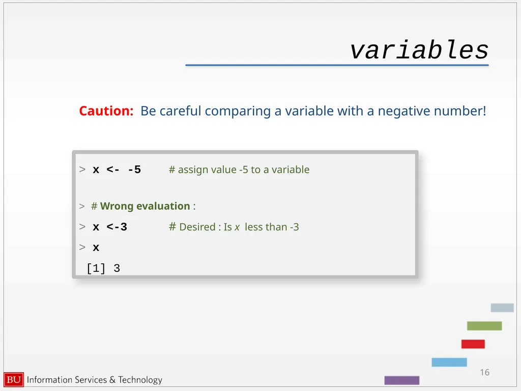
slide16. variables Caution: Be careful comparing a variable with a negative number! 16 > x <- -5 # assign value -5 to a variable

> # Wrong evaluation :
> x <-3 # Desired : Is x less than -3
> x
[1] 3<br>
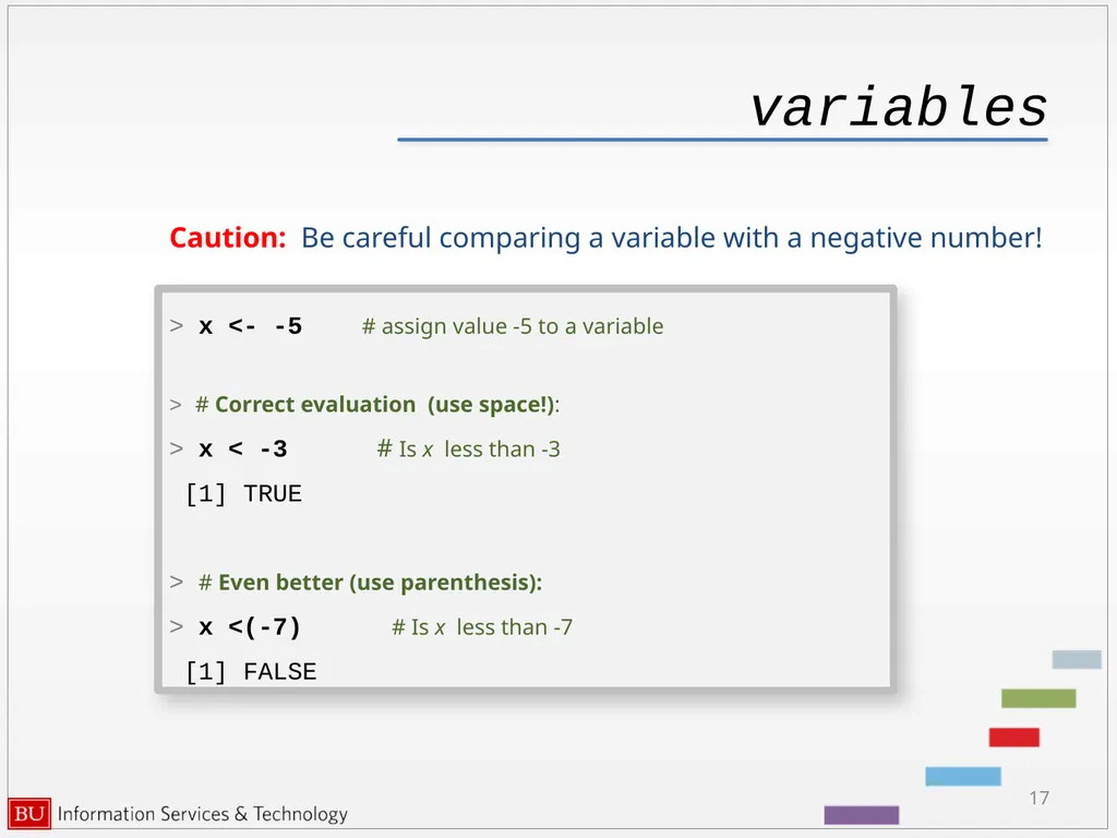
slide17. variables Caution: Be careful comparing a variable with a negative number! 17 > x <- -5 # assign value -5 to a variable

> # Correct evaluation (use space!):
> x < -3 # Is x less than -3
[1] TRUE

> # Even better (use parenthesis):
> x <(-7) # Is x less than -7
[1] FALSE<br>
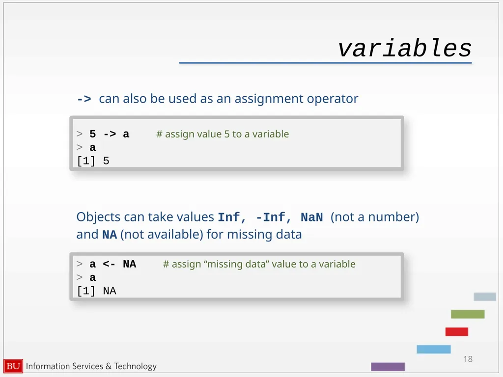
slide18. variables -> can also be used as an assignment operator

Objects can take values Inf, -Inf, NaN (not a number)
and NA (not available) for missing data 18 > 5 -> a # assign value 5 to a variable
> a
[1] 5 > a <- NA # assign “missing data” value to a variable
> a
[1] NA<br>
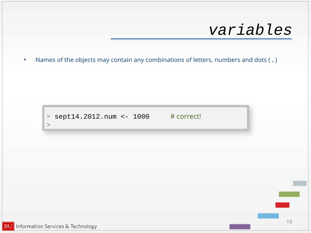
slide19. variables Names of the objects may contain any combinations of letters, numbers and dots ( . ) 19 > sept14.2012.num <- 1000 # correct!
><br>
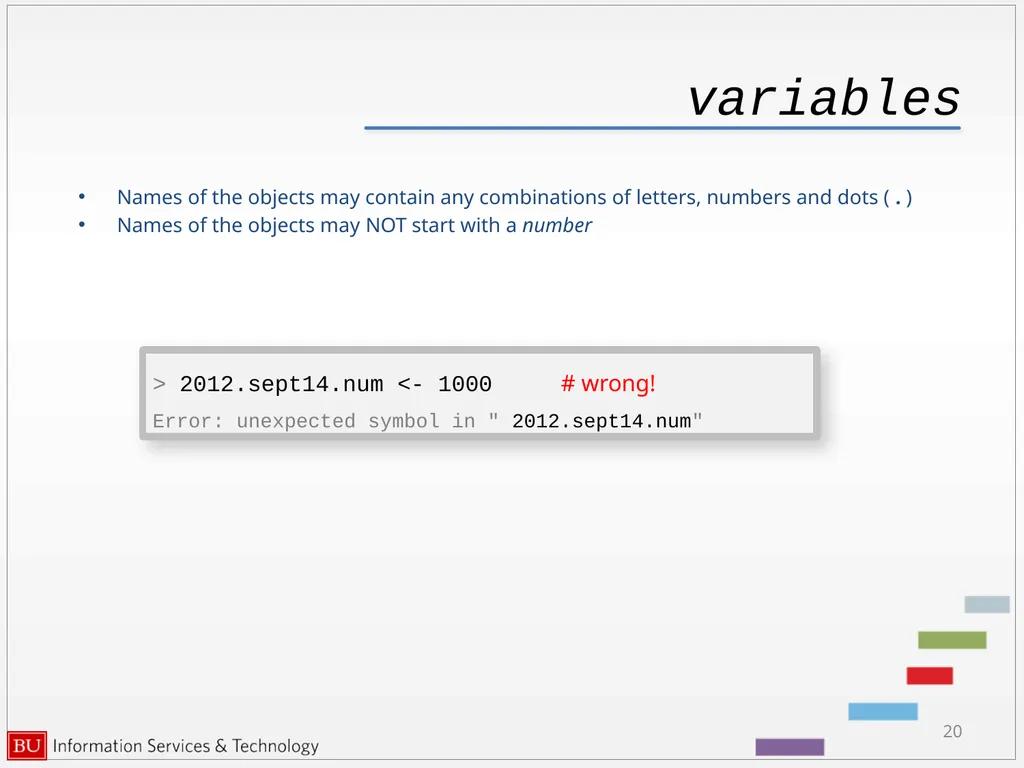
slide20. variables Names of the objects may contain any combinations of letters, numbers and dots ( . )
Names of the objects may NOT start with a number 20 > 2012.sept14.num <- 1000 # wrong!
Error: unexpected symbol in " 2012.sept14.num"<br>
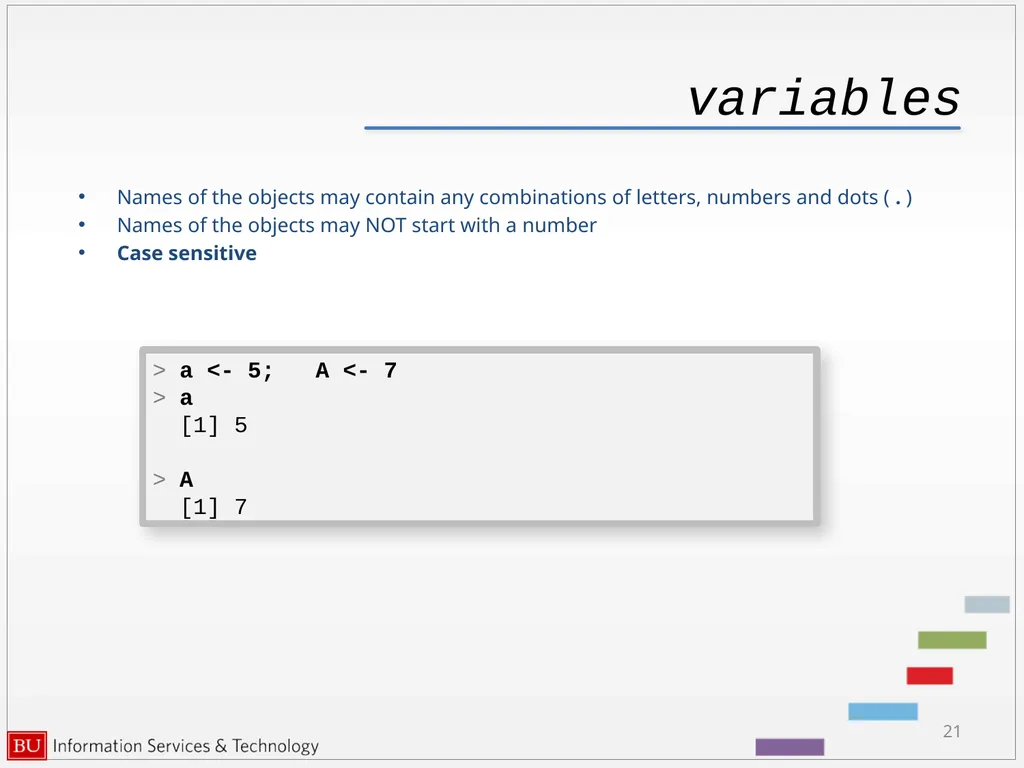
slide21. variables Names of the objects may contain any combinations of letters, numbers and dots ( . )
Names of the objects may NOT start with a number
Case sensitive 21 > a <- 5; A <- 7
> a
[1] 5

> A
[1] 7<br>
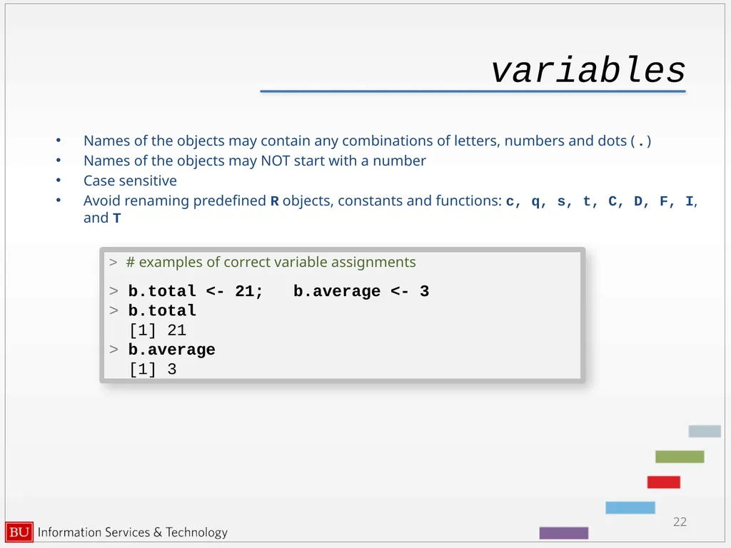
slide22. variables Names of the objects may contain any combinations of letters, numbers and dots ( . )
Names of the objects may NOT start with a number
Case sensitive
Avoid renaming predefined R objects, constants and functions: c, q, s, t, C, D, F, I, and T 22 > # examples of correct variable assignments
> b.total <- 21; b.average <- 3
> b.total
[1] 21
> b.average
[1] 3<br>
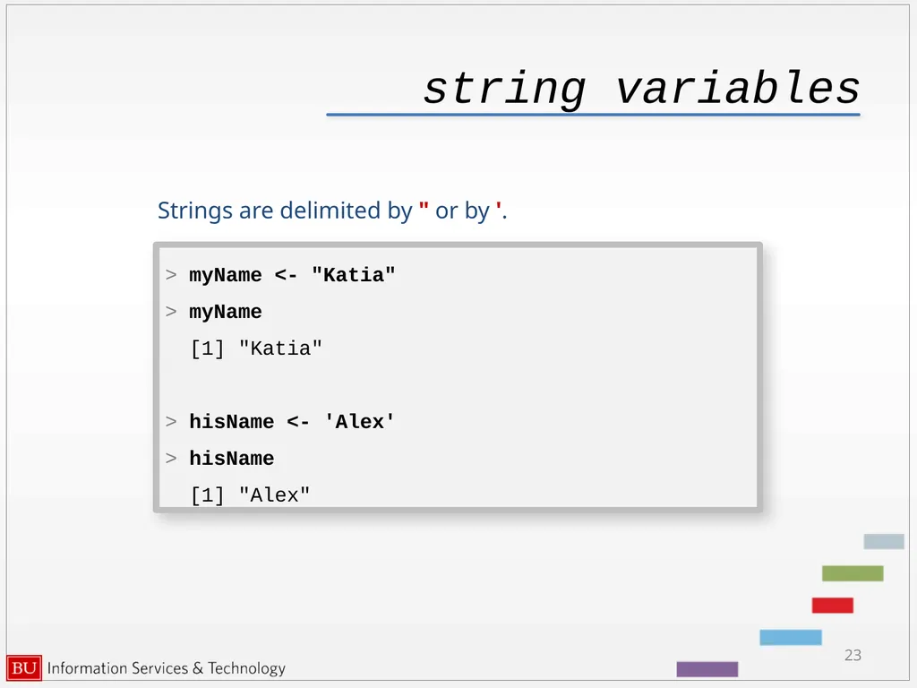
slide23. string variables Strings are delimited by " or by '. 23 > myName <- "Katia"
> myName
[1] "Katia"

> hisName <- 'Alex'
> hisName
[1] "Alex"<br>
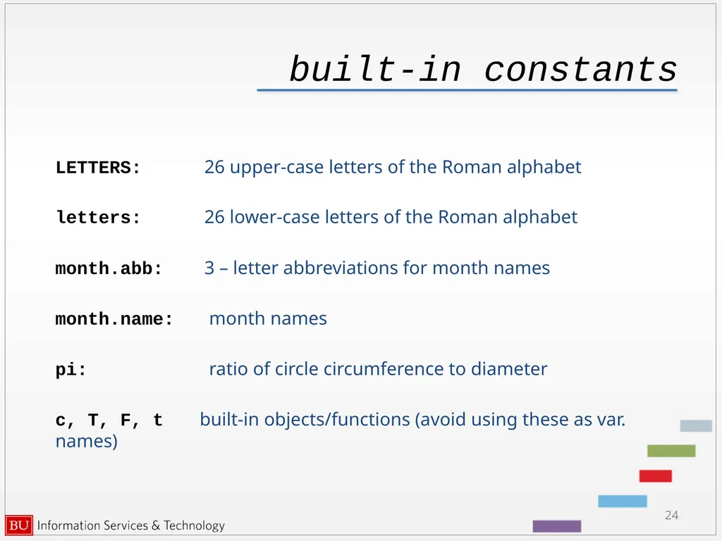
slide24. built-in constants LETTERS: 26 upper-case letters of the Roman alphabet

letters: 26 lower-case letters of the Roman alphabet

month.abb: 3 – letter abbreviations for month names

month.name: month names

pi: ratio of circle circumference to diameter

c, T, F, t built-in objects/functions (avoid using these as var. names) 24<br>
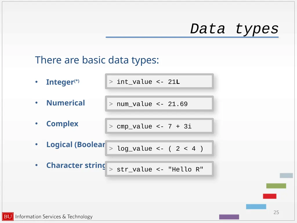
slide25. Data types There are basic data types:

Integer(*)

Numerical

Complex

Logical (Boolean)

Character string 25 > num_value <- 21.69 > cmp_value <- 7 + 3i > log_value <- ( 2 < 4 ) > str_value <- "Hello R" > int_value <- 21L<br>
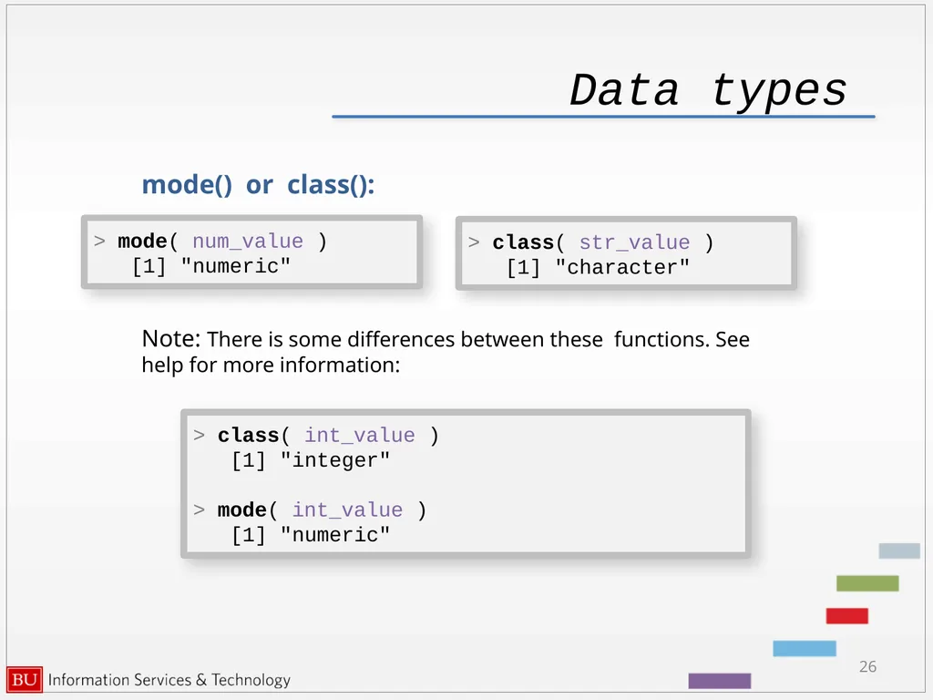
slide26. Data types mode() or class():

Note: There is some differences between these functions. See help for more information: 26 > mode( num_value )
[1] "numeric" > class( str_value )
[1] "character" > class( int_value )
[1] "integer"

> mode( int_value )
[1] "numeric"<br>
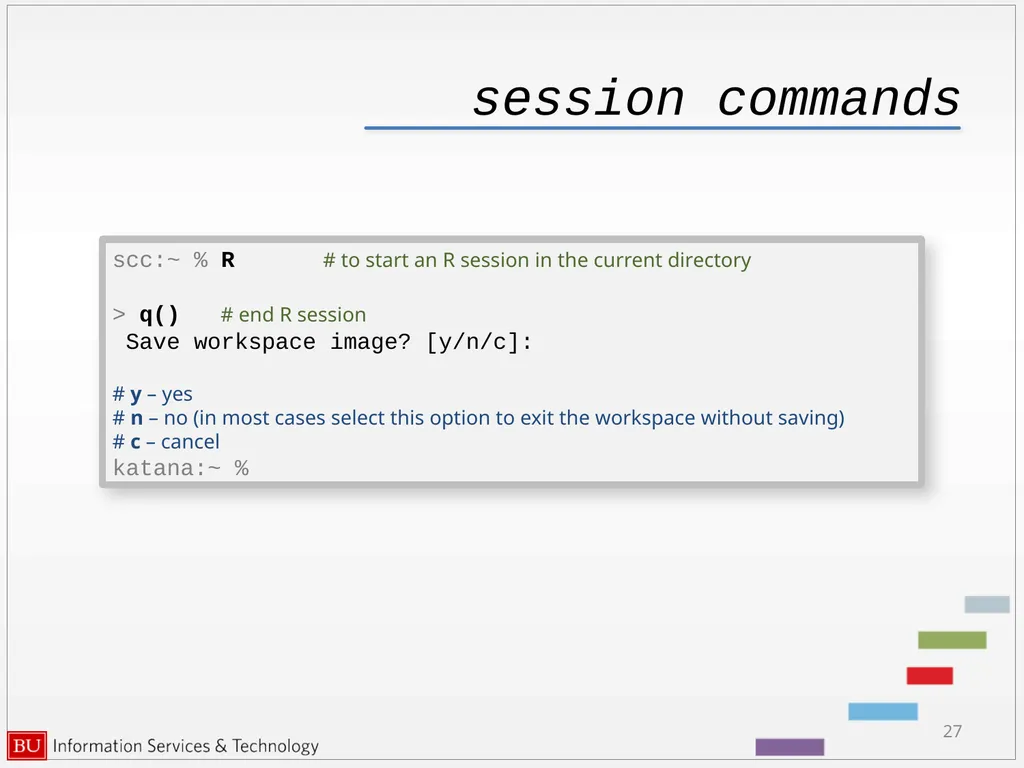
slide27. session commands 27 scc:~ % R # to start an R session in the current directory

> q() # end R session
Save workspace image? [y/n/c]:

# y – yes
# n – no (in most cases select this option to exit the workspace without saving)
# c – cancel
katana:~ %<br>
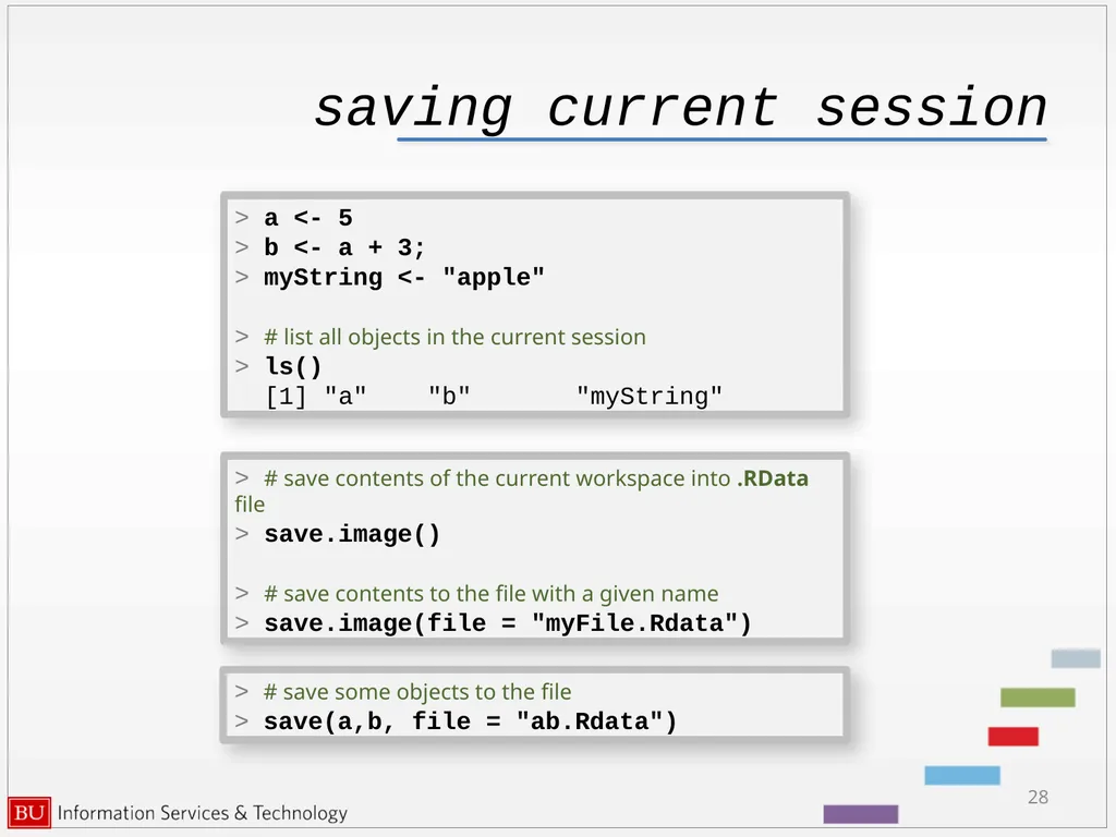
slide28. saving current session 28 > a <- 5
> b <- a + 3;
> myString <- "apple"

> # list all objects in the current session
> ls()
[1] "a" "b" "myString" > # save contents of the current workspace into .RData file
> save.image()

> # save contents to the file with a given name
> save.image(file = "myFile.Rdata") > # save some objects to the file
> save(a,b, file = "ab.Rdata")<br>
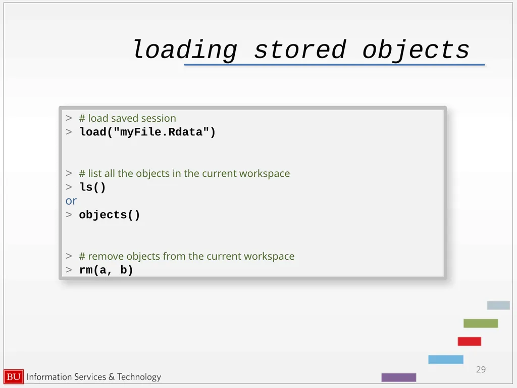
slide29. loading stored objects 29 > # load saved session
> load("myFile.Rdata")

> # list all the objects in the current workspace
> ls()
or
> objects()


> # remove objects from the current workspace
> rm(a, b)<br>
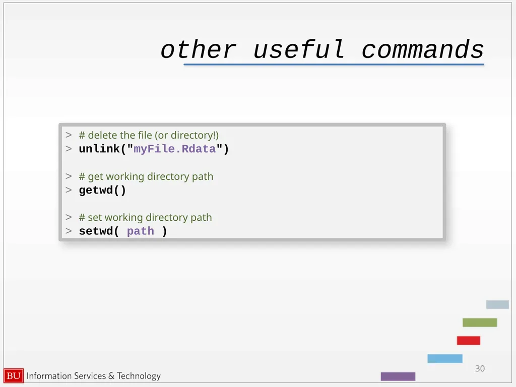
slide30. other useful commands 30 > # delete the file (or directory!)
> unlink("myFile.Rdata")

> # get working directory path
> getwd()

> # set working directory path
> setwd( path )<br>
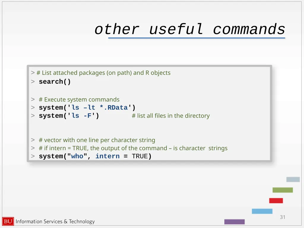
slide31. other useful commands 31 > # List attached packages (on path) and R objects
> search()

> # Execute system commands
> system('ls –lt *.RData')
> system('ls -F') # list all files in the directory

> # vector with one line per character string
> # if intern = TRUE, the output of the command – is character strings
> system("who", intern = TRUE)<br>
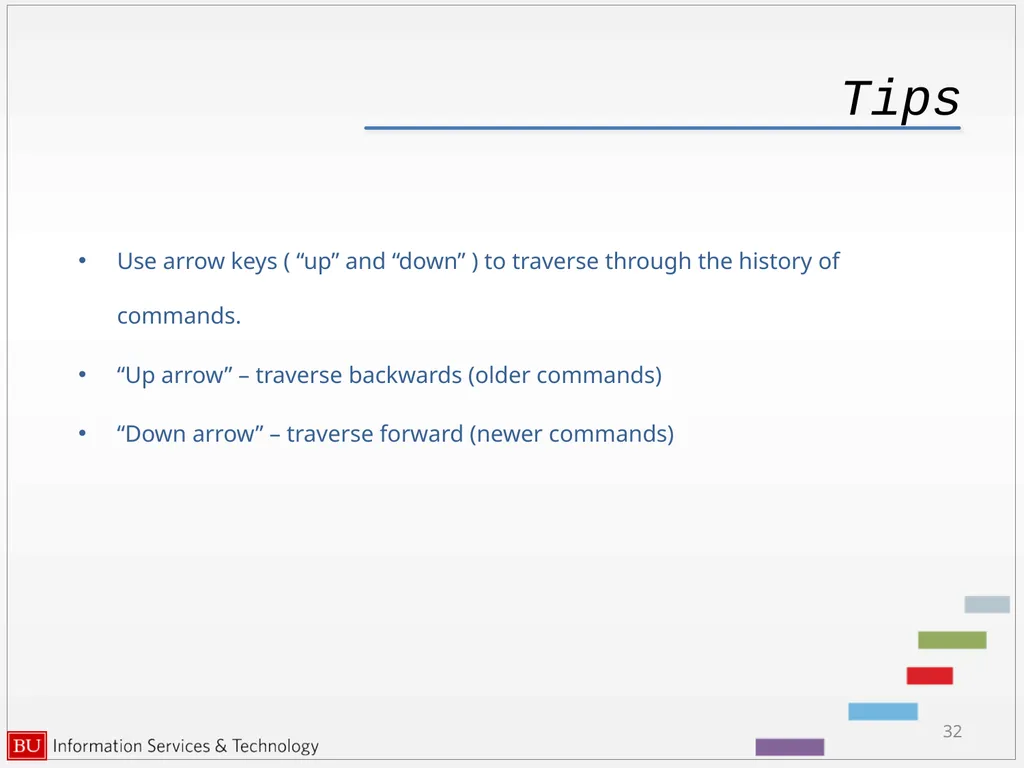
slide32. Tips Use arrow keys ( “up” and “down” ) to traverse through the history of commands.
“Up arrow” – traverse backwards (older commands)
“Down arrow” – traverse forward (newer commands) 32<br>
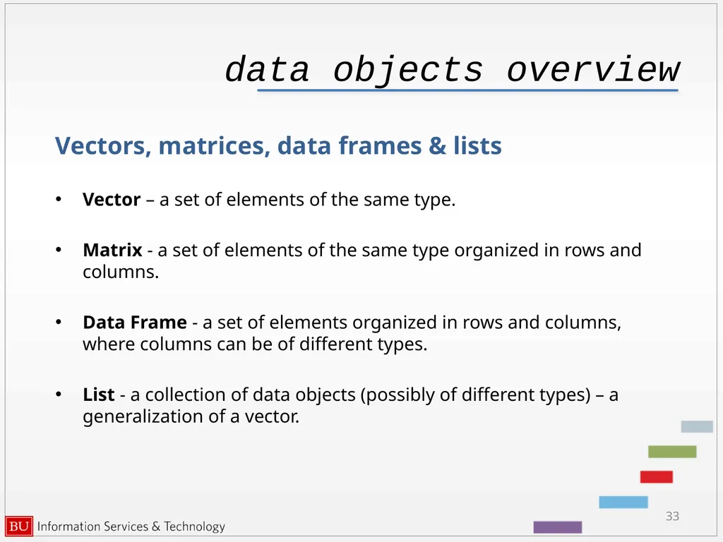
slide33. data objects overview Vectors, matrices, data frames & lists

Vector – a set of elements of the same type.

Matrix - a set of elements of the same type organized in rows and columns.

Data Frame - a set of elements organized in rows and columns, where columns can be of different types.

List - a collection of data objects (possibly of different types) – a generalization of a vector. 33<br>
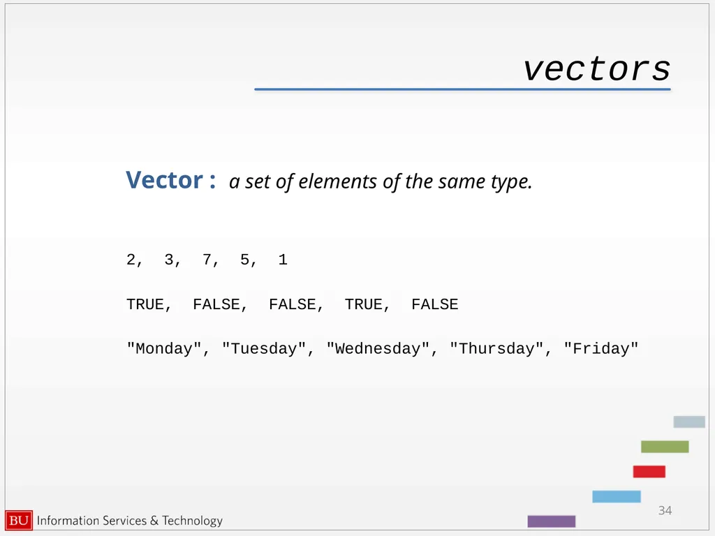
slide34. vectors Vector : a set of elements of the same type.

2, 3, 7, 5, 1

TRUE, FALSE, FALSE, TRUE, FALSE

"Monday", "Tuesday", "Wednesday", "Thursday", "Friday" 34<br>
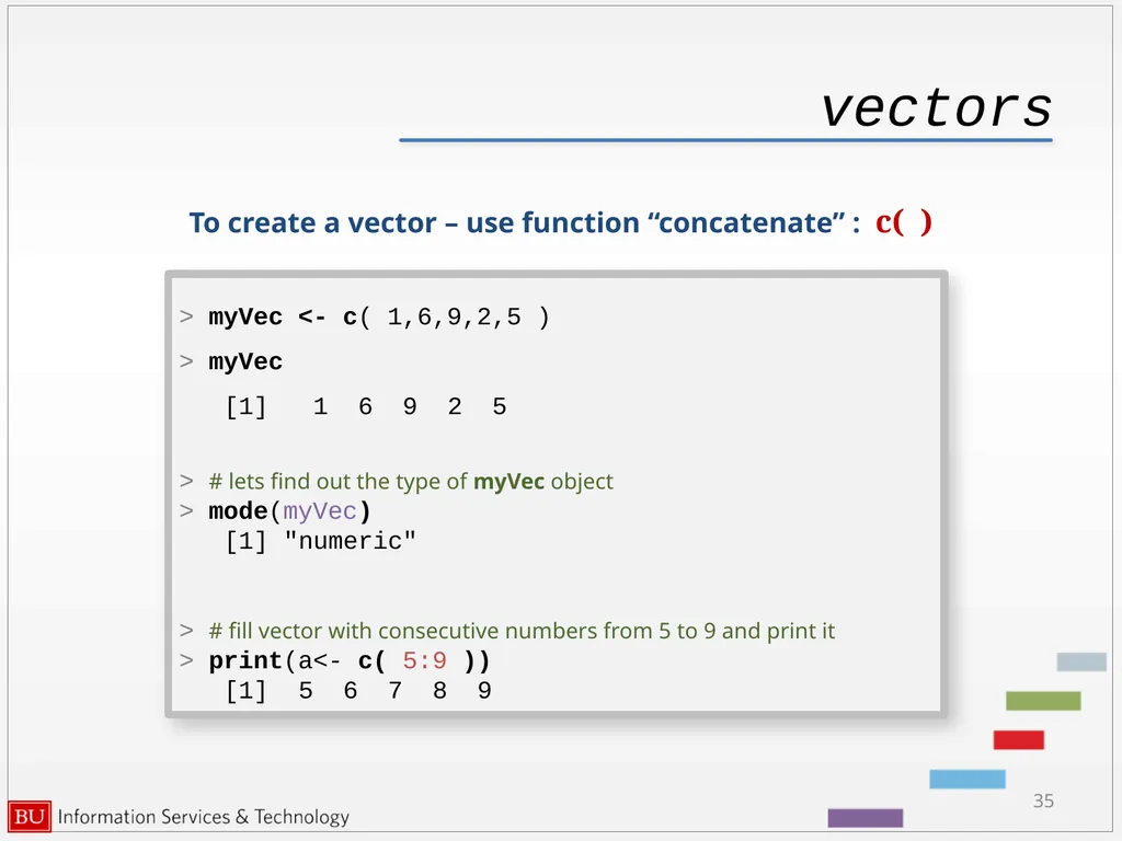
slide35. vectors To create a vector – use function “concatenate” : c( ) 35 > myVec <- c( 1,6,9,2,5 )
> myVec
[1] 1 6 9 2 5

> # lets find out the type of myVec object
> mode(myVec)
[1] "numeric"

> # fill vector with consecutive numbers from 5 to 9 and print it
> print(a<- c( 5:9 ))
[1] 5 6 7 8 9<br>
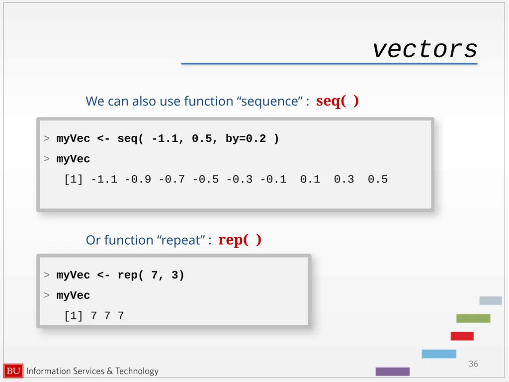
slide36. vectors We can also use function “sequence” : seq( ) 36 > myVec <- seq( -1.1, 0.5, by=0.2 )
> myVec
[1] -1.1 -0.9 -0.7 -0.5 -0.3 -0.1 0.1 0.3 0.5 Or function “repeat” : rep( ) > myVec <- rep( 7, 3)
> myVec
[1] 7 7 7<br>
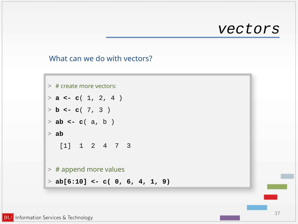
slide37. vectors What can we do with vectors? 37 > # create more vectors:
> a <- c( 1, 2, 4 )
> b <- c( 7, 3 )
> ab <- c( a, b )
> ab
[1] 1 2 4 7 3

> # append more values
> ab[6:10] <- c( 0, 6, 4, 1, 9)<br>
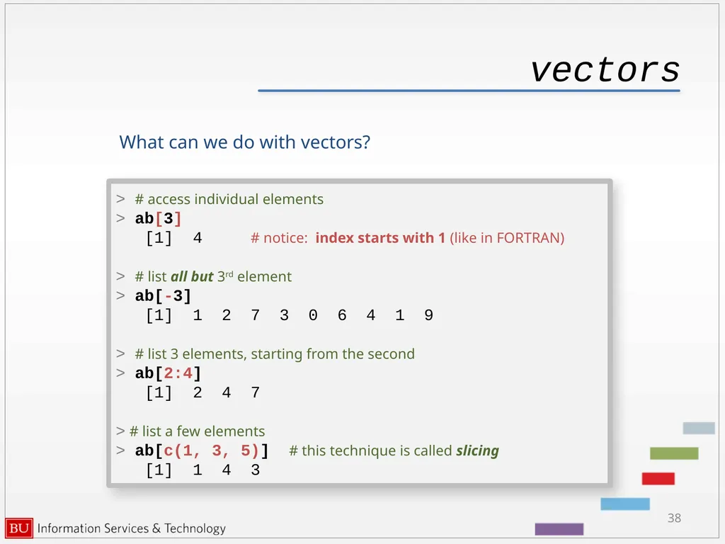
slide38. vectors What can we do with vectors? 38 > # access individual elements
> ab[3]
[1] 4 # notice: index starts with 1 (like in FORTRAN)

> # list all but 3rd element
> ab[-3]
[1] 1 2 7 3 0 6 4 1 9

> # list 3 elements, starting from the second
> ab[2:4]
[1] 2 4 7

> # list a few elements
> ab[c(1, 3, 5)] # this technique is called slicing
[1] 1 4 3<br>
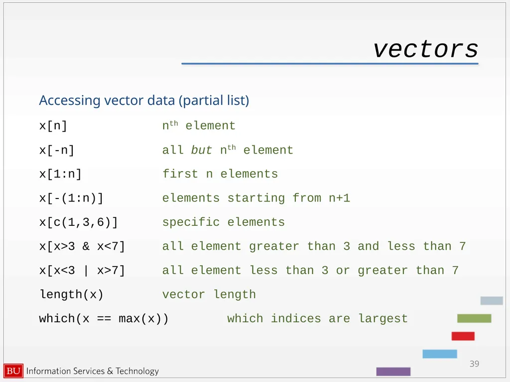
slide39. vectors Accessing vector data (partial list)
x[n] nth element
x[-n] all but nth element
x[1:n] first n elements
x[-(1:n)] elements starting from n+1
x[c(1,3,6)] specific elements
x[x>3 & x<7] all element greater than 3 and less than 7
x[x<3 | x>7] all element less than 3 or greater than 7
length(x) vector length
which(x == max(x)) which indices are largest 39<br>
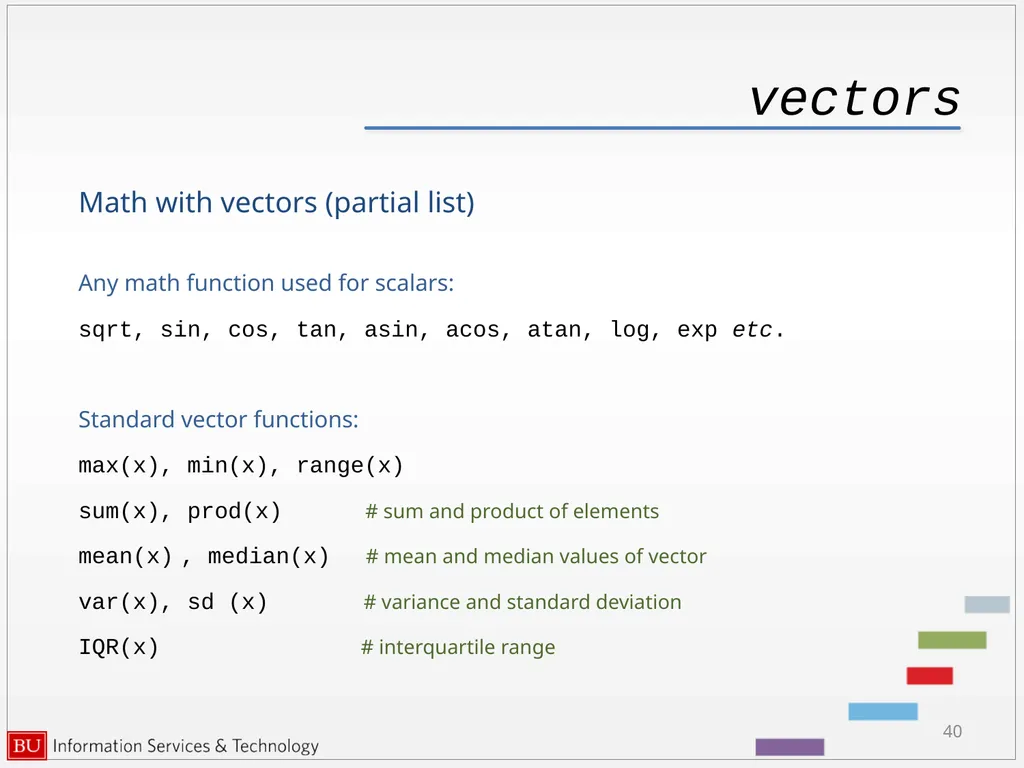
slide40. vectors Math with vectors (partial list)

Any math function used for scalars:
sqrt, sin, cos, tan, asin, acos, atan, log, exp etc.

Standard vector functions:
max(x), min(x), range(x)
sum(x), prod(x) # sum and product of elements
mean(x) , median(x) # mean and median values of vector
var(x), sd (x) # variance and standard deviation
IQR(x) # interquartile range 40<br>
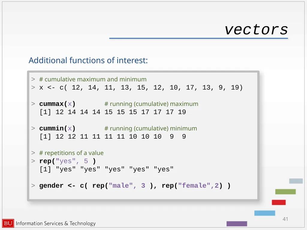
slide41. vectors Additional functions of interest: 41 > # cumulative maximum and minimum
> x <- c( 12, 14, 11, 13, 15, 12, 10, 17, 13, 9, 19)

> cummax(x) # running (cumulative) maximum
[1] 12 14 14 14 15 15 15 17 17 17 19

> cummin(x) # running (cumulative) minimum
[1] 12 12 11 11 11 11 10 10 10 9 9

> # repetitions of a value
> rep("yes", 5 )
[1] "yes" "yes" "yes" "yes" "yes"

> gender <- c( rep("male", 3 ), rep("female",2) )<br>
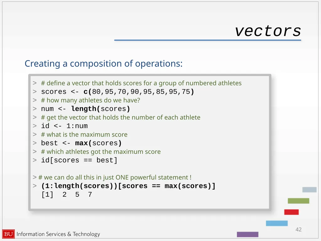
slide42. vectors Creating a composition of operations: 42 > # define a vector that holds scores for a group of numbered athletes
> scores <- c(80,95,70,90,95,85,95,75)
> # how many athletes do we have?
> num <- length(scores)
> # get the vector that holds the number of each athlete
> id <- 1:num
> # what is the maximum score
> best <- max(scores)
> # which athletes got the maximum score
> id[scores == best]

> # we can do all this in just ONE powerful statement !
> (1:length(scores))[scores == max(scores)]
[1] 2 5 7<br>
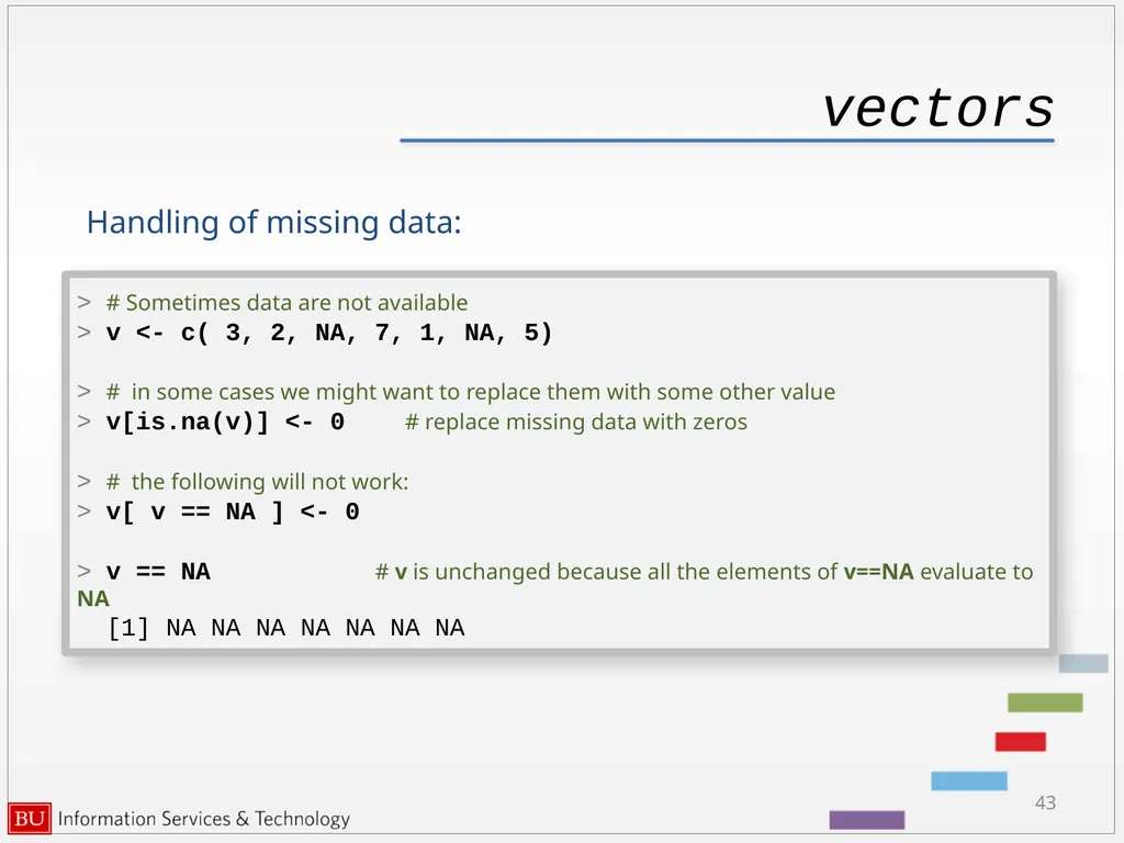
slide43. vectors Handling of missing data: 43 > # Sometimes data are not available
> v <- c( 3, 2, NA, 7, 1, NA, 5)

> # in some cases we might want to replace them with some other value
> v[is.na(v)] <- 0 # replace missing data with zeros

> # the following will not work:
> v[ v == NA ] <- 0

> v == NA # v is unchanged because all the elements of v==NA evaluate to NA
[1] NA NA NA NA NA NA NA<br>
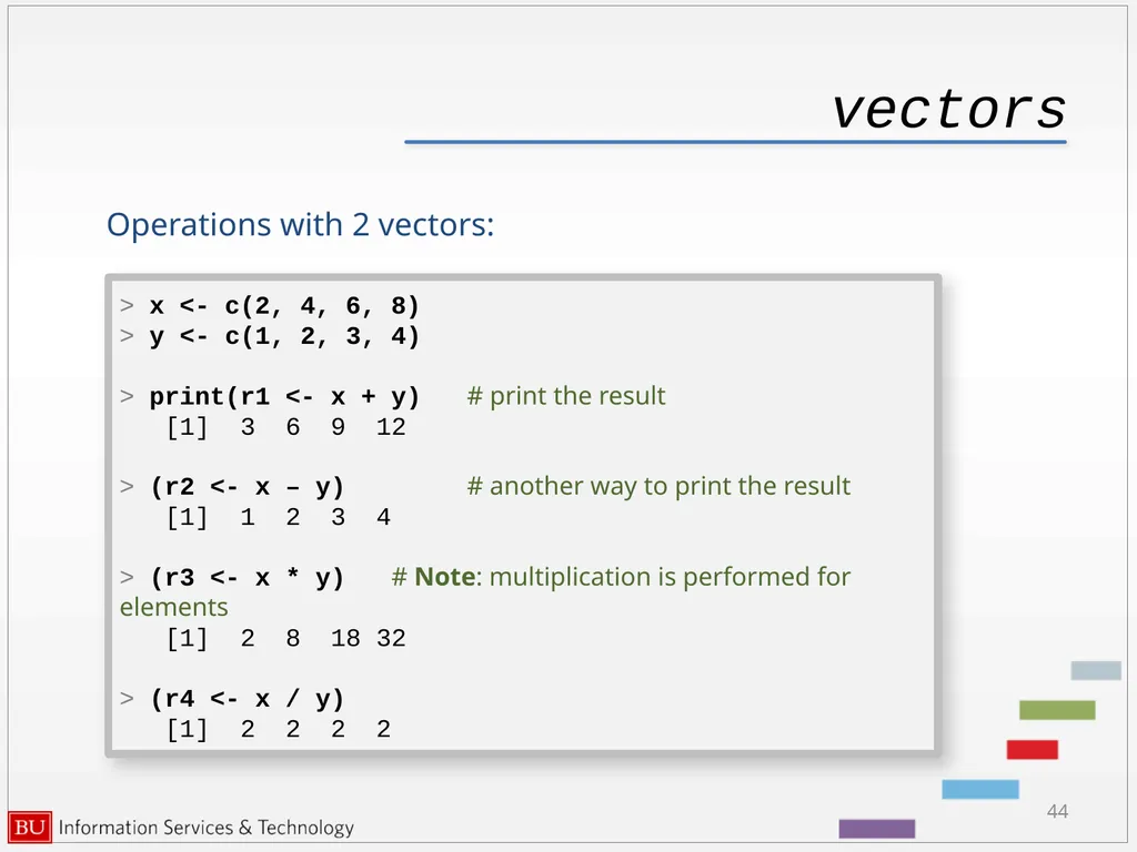
slide44. vectors Operations with 2 vectors: 44 > x <- c(2, 4, 6, 8)
> y <- c(1, 2, 3, 4)

> print(r1 <- x + y) # print the result
[1] 3 6 9 12

> (r2 <- x – y) # another way to print the result
[1] 1 2 3 4

> (r3 <- x * y) # Note: multiplication is performed for elements
[1] 2 8 18 32

> (r4 <- x / y)
[1] 2 2 2 2<br>
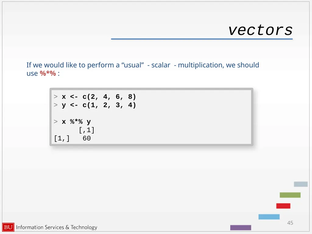
slide45. vectors 45 > x <- c(2, 4, 6, 8)
> y <- c(1, 2, 3, 4)

> x %*% y
[,1]
[1,] 60 If we would like to perform a “usual” - scalar - multiplication, we should use %*% :<br>
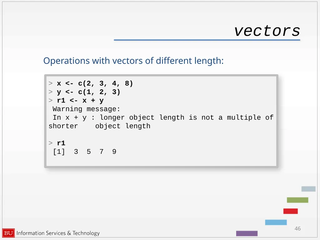
slide46. vectors Operations with vectors of different length: 46 > x <- c(2, 3, 4, 8)
> y <- c(1, 2, 3)
> r1 <- x + y
Warning message:
In x + y : longer object length is not a multiple of shorter object length

> r1
[1] 3 5 7 9<br>
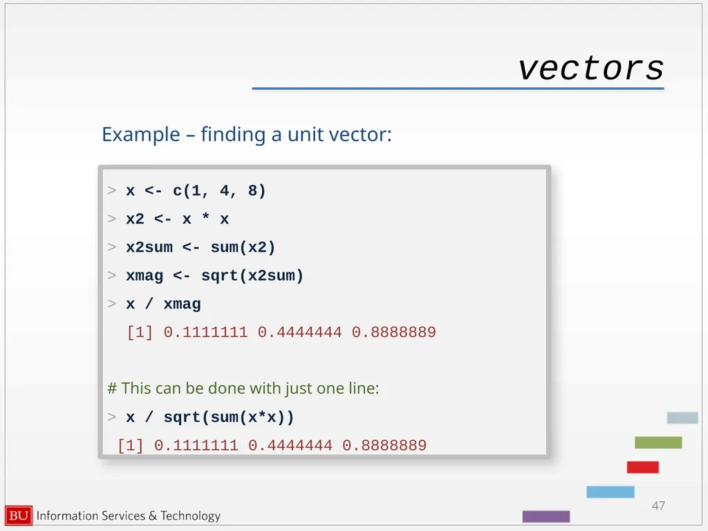
slide47. vectors Example – finding a unit vector: 47 > x <- c(1, 4, 8)
> x2 <- x * x
> x2sum <- sum(x2)
> xmag <- sqrt(x2sum)
> x / xmag
[1] 0.1111111 0.4444444 0.8888889

# This can be done with just one line:
> x / sqrt(sum(x*x))
[1] 0.1111111 0.4444444 0.8888889<br>
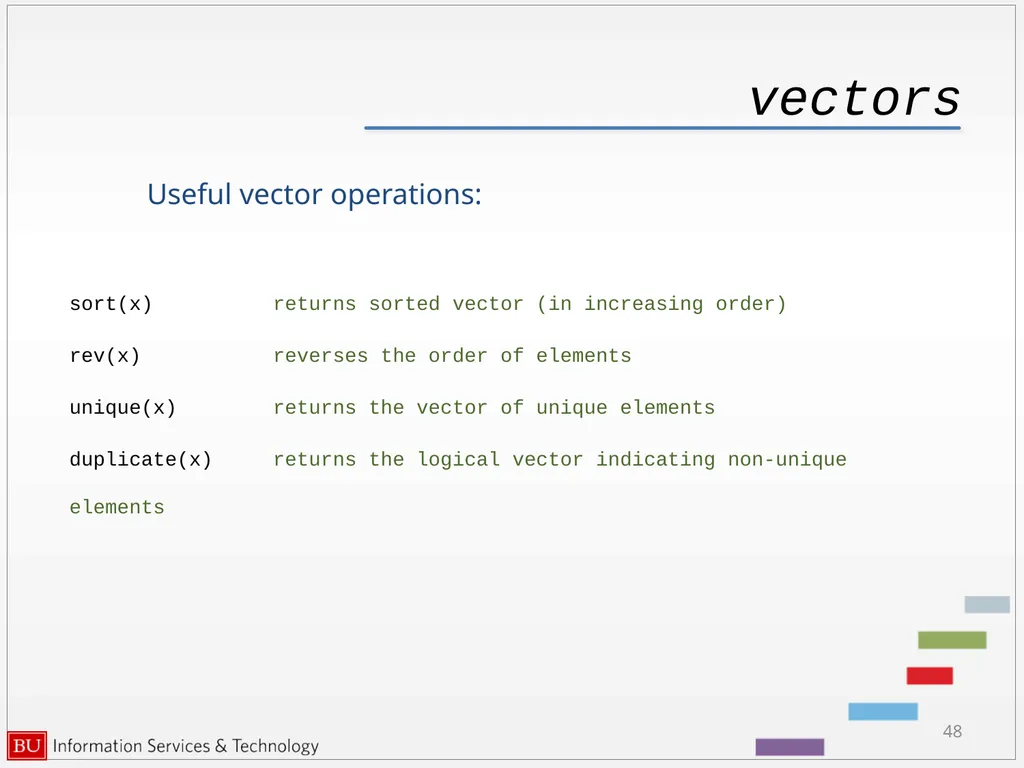
slide48. vectors Useful vector operations: 48 sort(x) returns sorted vector (in increasing order)
rev(x) reverses the order of elements
unique(x) returns the vector of unique elements
duplicate(x) returns the logical vector indicating non-unique elements<br>
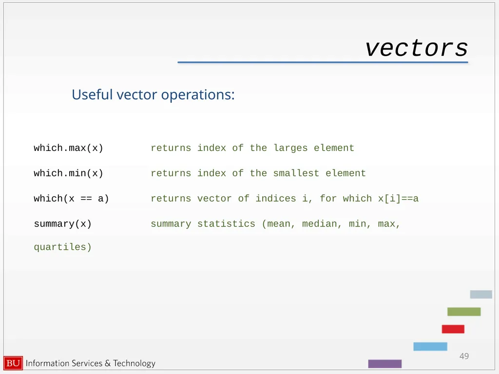
slide49. vectors Useful vector operations: 49 which.max(x) returns index of the larges element
which.min(x) returns index of the smallest element
which(x == a) returns vector of indices i, for which x[i]==a
summary(x) summary statistics (mean, median, min, max, quartiles)<br>
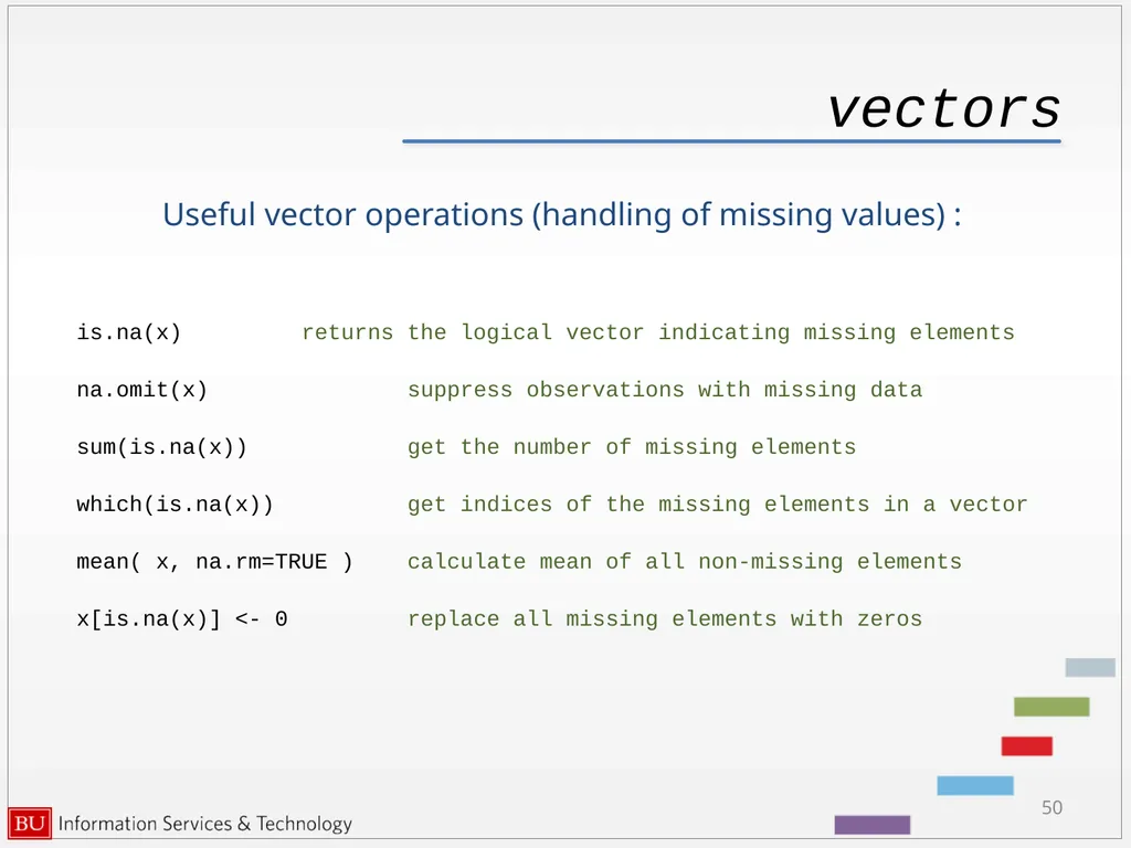
slide50. vectors Useful vector operations (handling of missing values) : 50 is.na(x) returns the logical vector indicating missing elements
na.omit(x) suppress observations with missing data
sum(is.na(x)) get the number of missing elements
which(is.na(x)) get indices of the missing elements in a vector
mean( x, na.rm=TRUE ) calculate mean of all non-missing elements
x[is.na(x)] <- 0 replace all missing elements with zeros<br>
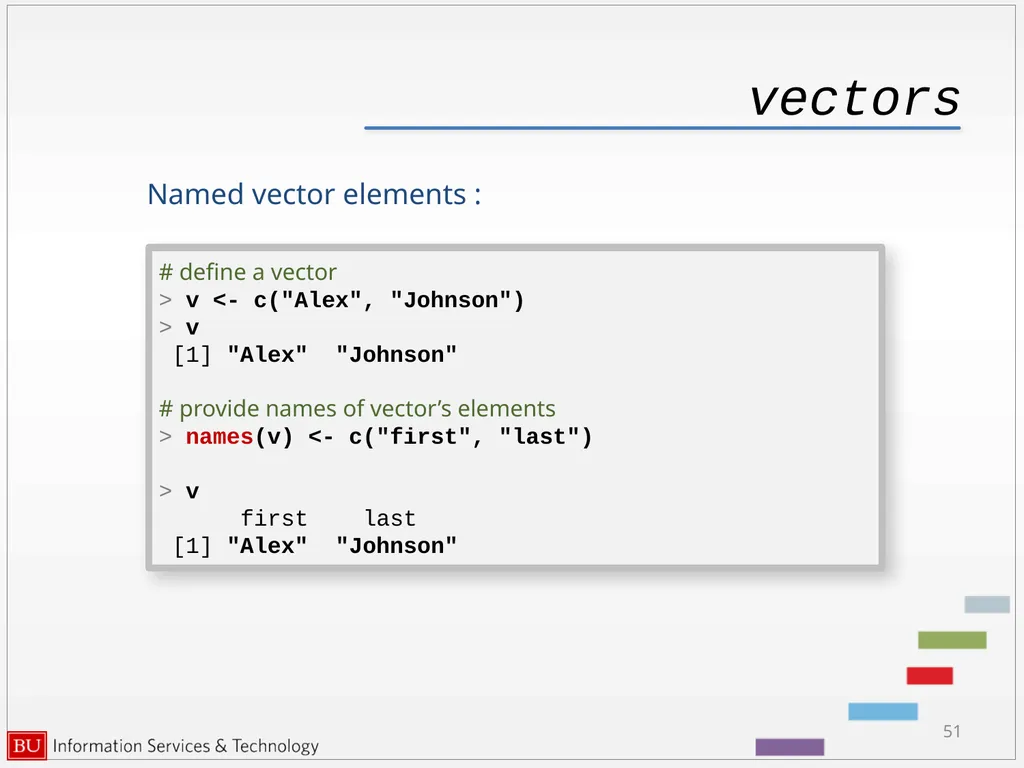
slide51. vectors Named vector elements : 51 # define a vector
> v <- c("Alex", "Johnson")
> v
[1] "Alex" "Johnson"

# provide names of vector’s elements
> names(v) <- c("first", "last")

> v
first last
[1] "Alex" "Johnson"<br>
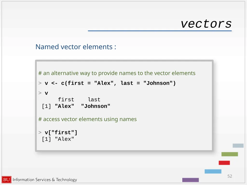
slide52. vectors Named vector elements : 52 # an alternative way to provide names to the vector elements
> v <- c(first = "Alex", last = "Johnson")
> v
first last
[1] "Alex" "Johnson"

# access vector elements using names
> v["first"]
[1] "Alex"<br>
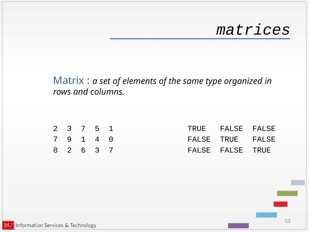
slide53. matrices Matrix : a set of elements of the same type organized in rows and columns.

2 3 7 5 1 TRUE FALSE FALSE
7 9 1 4 0 FALSE TRUE FALSE
8 2 6 3 7 FALSE FALSE TRUE 53<br>
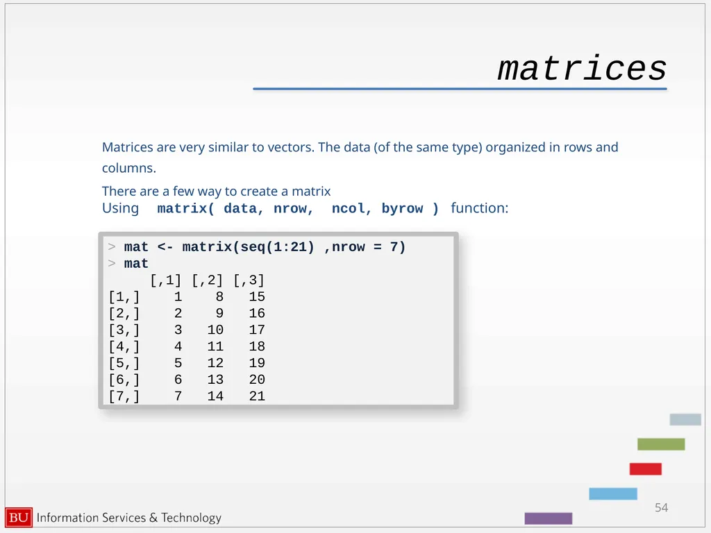
slide54. matrices Matrices are very similar to vectors. The data (of the same type) organized in rows and columns.
There are a few way to create a matrix 54 Using matrix( data, nrow, ncol, byrow ) function: > mat <- matrix(seq(1:21) ,nrow = 7)
> mat
[,1] [,2] [,3]
[1,] 1 8 15
[2,] 2 9 16
[3,] 3 10 17
[4,] 4 11 18
[5,] 5 12 19
[6,] 6 13 20
[7,] 7 14 21<br>
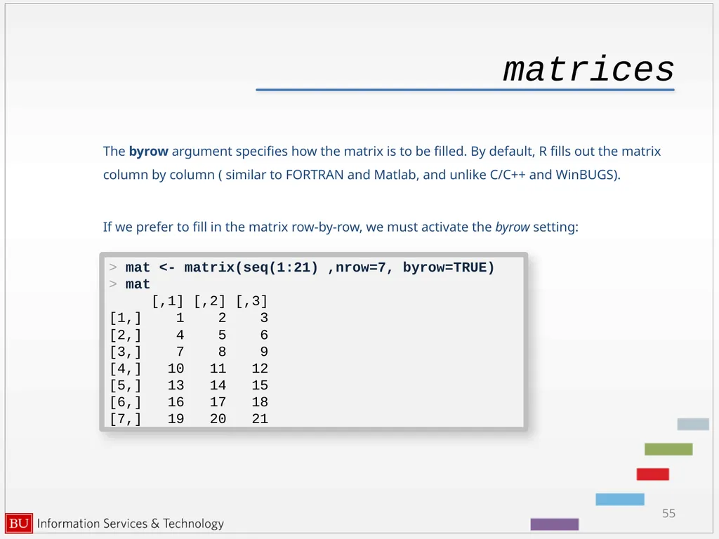
slide55. matrices The byrow argument specifies how the matrix is to be filled. By default, R fills out the matrix column by column ( similar to FORTRAN and Matlab, and unlike C/C++ and WinBUGS).

If we prefer to fill in the matrix row-by-row, we must activate the byrow setting: 55 > mat <- matrix(seq(1:21) ,nrow=7, byrow=TRUE)
> mat
[,1] [,2] [,3]
[1,] 1 2 3
[2,] 4 5 6
[3,] 7 8 9
[4,] 10 11 12
[5,] 13 14 15
[6,] 16 17 18
[7,] 19 20 21<br>
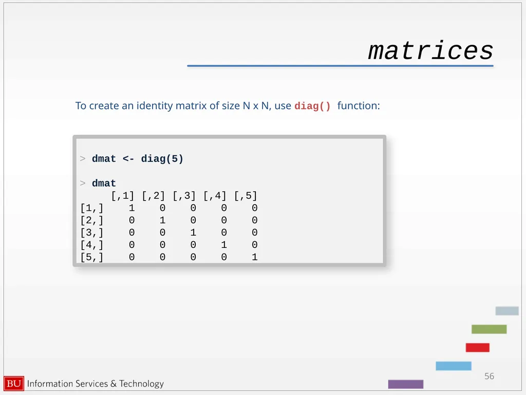
slide56. matrices To create an identity matrix of size N x N, use diag() function: 56 > dmat <- diag(5)
> dmat
[,1] [,2] [,3] [,4] [,5]
[1,] 1 0 0 0 0
[2,] 0 1 0 0 0
[3,] 0 0 1 0 0
[4,] 0 0 0 1 0
[5,] 0 0 0 0 1<br>
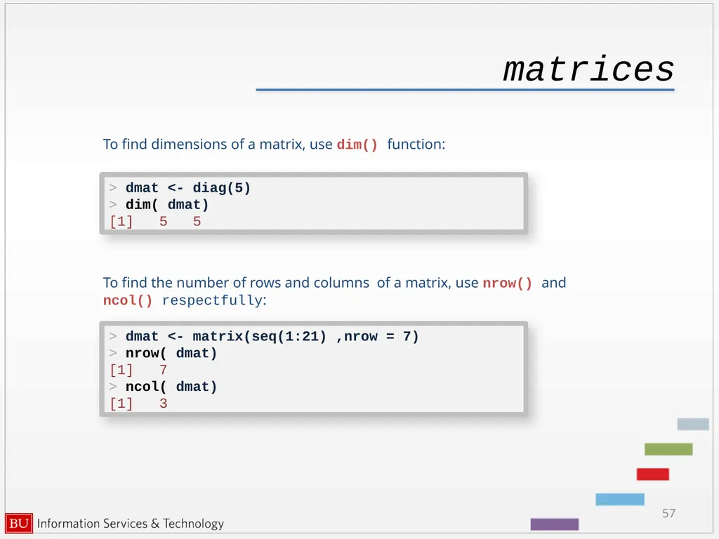
slide57. matrices To find dimensions of a matrix, use dim() function: 57 > dmat <- diag(5)
> dim( dmat)
[1] 5 5 To find the number of rows and columns of a matrix, use nrow() and ncol() respectfully: > dmat <- matrix(seq(1:21) ,nrow = 7)
> nrow( dmat)
[1] 7
> ncol( dmat)
[1] 3<br>
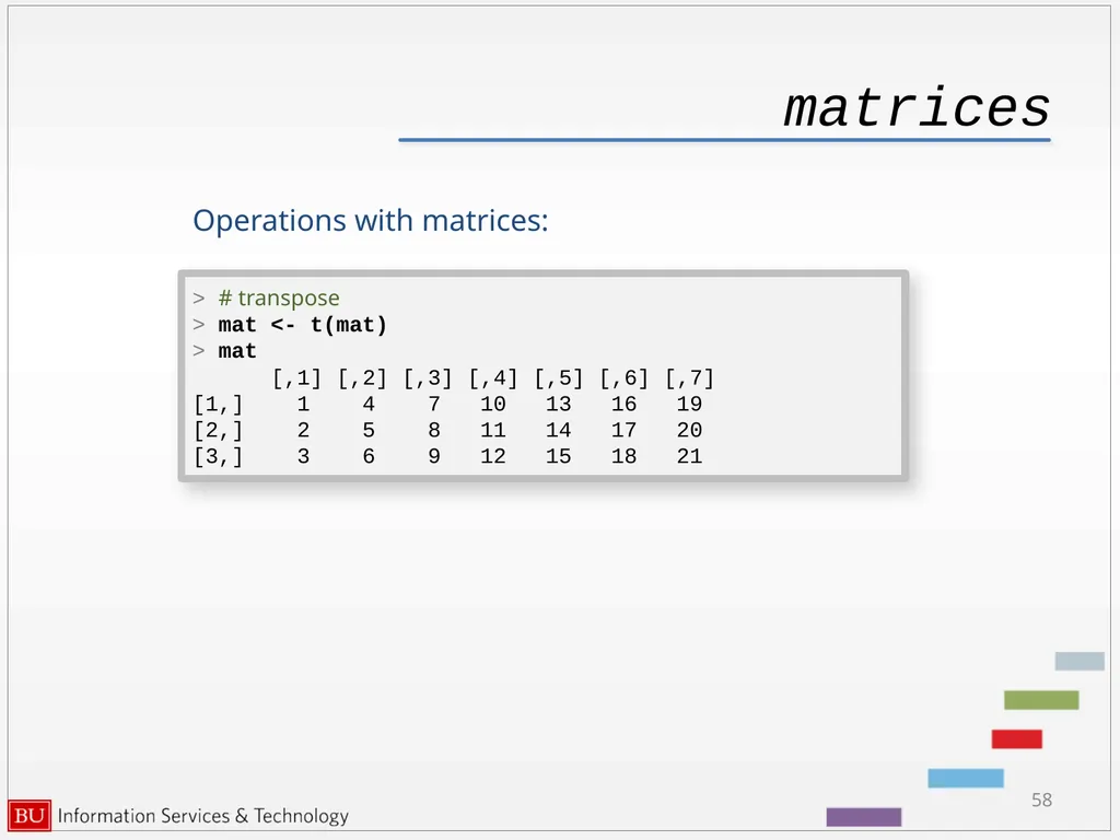
slide58. matrices Operations with matrices: 58 > # transpose
> mat <- t(mat)
> mat
[,1] [,2] [,3] [,4] [,5] [,6] [,7]
[1,] 1 4 7 10 13 16 19
[2,] 2 5 8 11 14 17 20
[3,] 3 6 9 12 15 18 21<br>
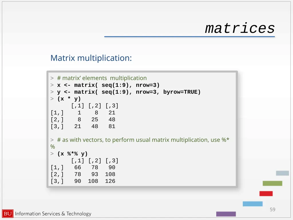
slide59. matrices Matrix multiplication: 59 > # matrix’ elements multiplication
> x <- matrix( seq(1:9), nrow=3)
> y <- matrix( seq(1:9), nrow=3, byrow=TRUE)
> (x * y)
[,1] [,2] [,3]
[1,] 1 8 21
[2,] 8 25 48
[3,] 21 48 81

> # as with vectors, to perform usual matrix multiplication, use %*%
> (x %*% y)
[,1] [,2] [,3]
[1,] 66 78 90
[2,] 78 93 108
[3,] 90 108 126<br>
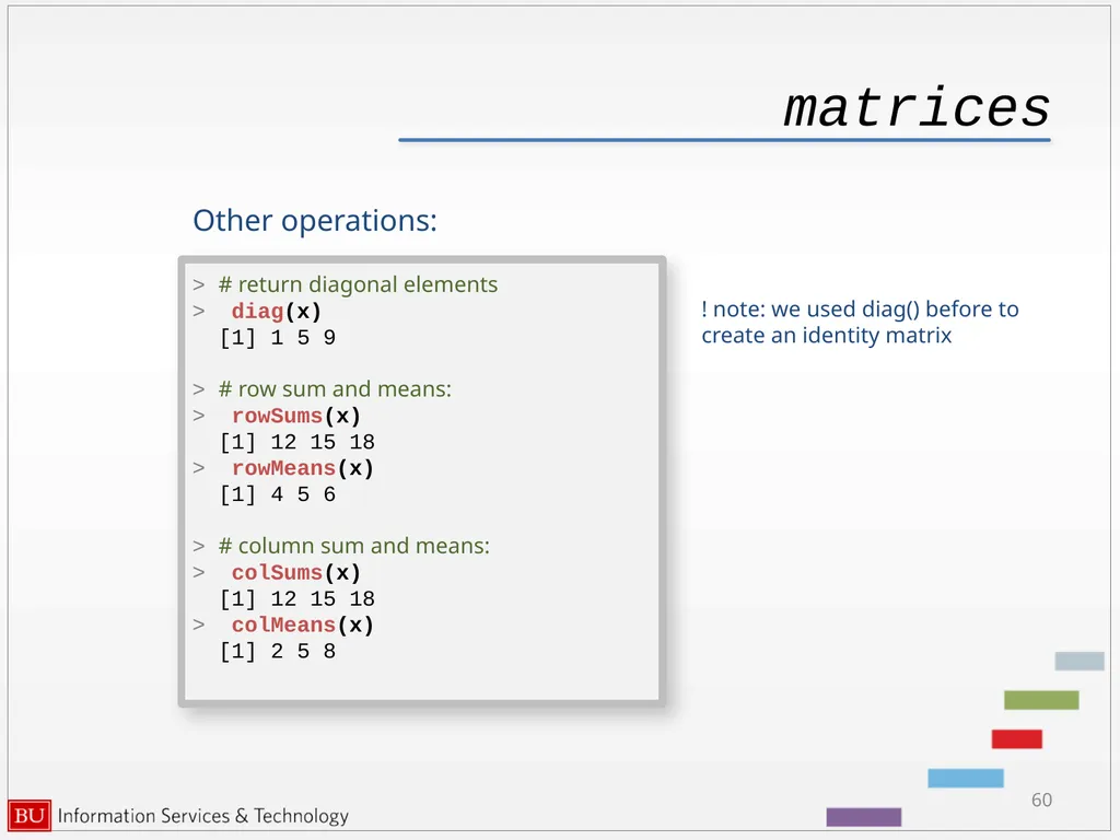
slide60. matrices Other operations: 60 > # return diagonal elements
> diag(x)
[1] 1 5 9

> # row sum and means:
> rowSums(x)
[1] 12 15 18
> rowMeans(x)
[1] 4 5 6

> # column sum and means:
> colSums(x)
[1] 12 15 18
> colMeans(x)
[1] 2 5 8 ! note: we used diag() before to create an identity matrix<br>
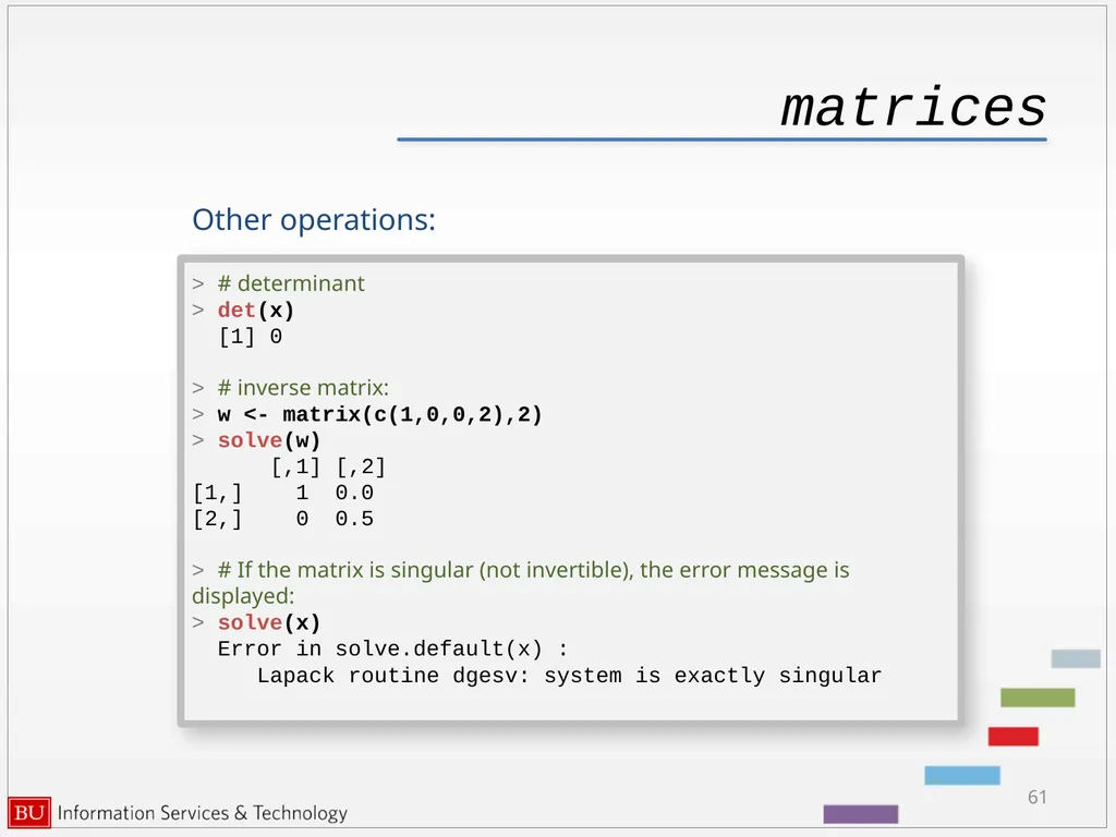
slide61. matrices Other operations: 61 > # determinant
> det(x)
[1] 0

> # inverse matrix:
> w <- matrix(c(1,0,0,2),2)
> solve(w)
[,1] [,2]
[1,] 1 0.0
[2,] 0 0.5

> # If the matrix is singular (not invertible), the error message is displayed:
> solve(x)
Error in solve.default(x) :
Lapack routine dgesv: system is exactly singular<br>
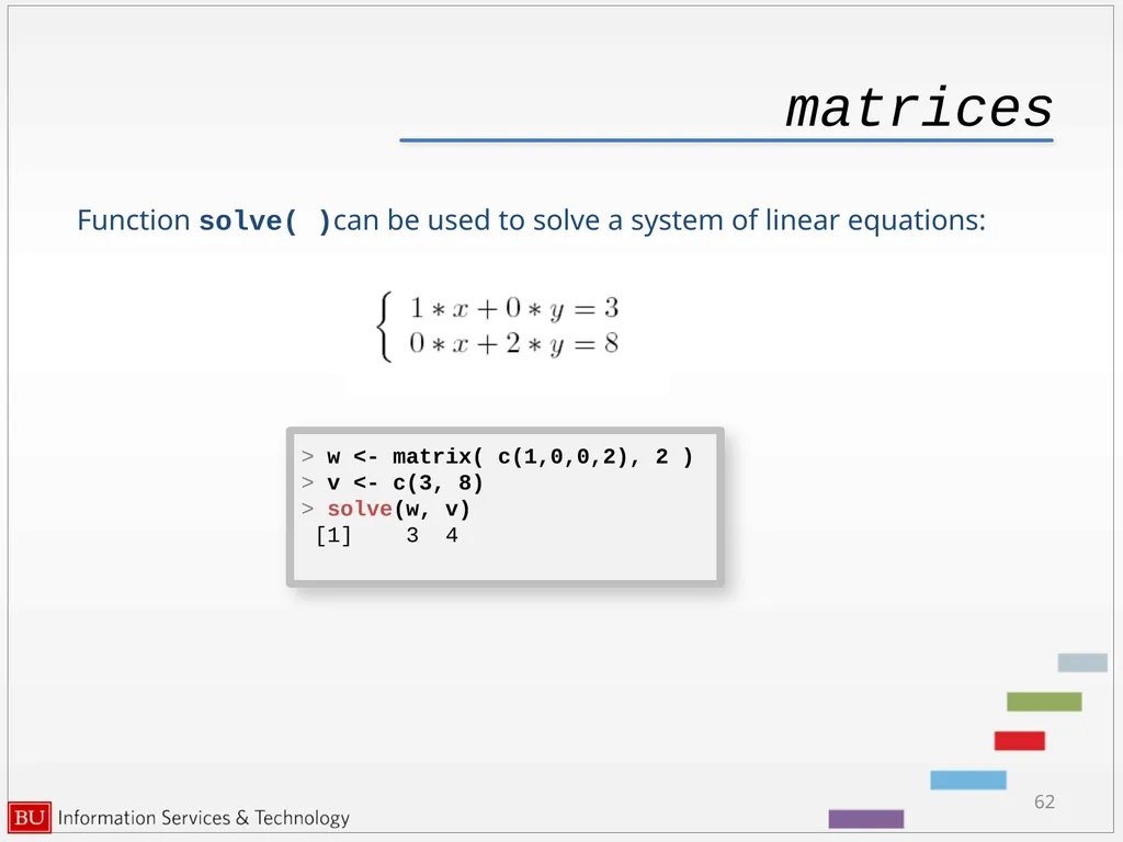
slide62. matrices Function solve( )can be used to solve a system of linear equations: 62 > w <- matrix( c(1,0,0,2), 2 )
> v <- c(3, 8)
> solve(w, v)
[1] 3 4<br>
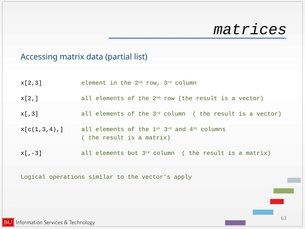
slide63. matrices 63 Accessing matrix data (partial list)

x[2,3] element in the 2nd row, 3rd column
x[2,] all elements of the 2nd row (the result is a vector)
x[,3] all elements of the 3rd column ( the result is a vector)
x[c(1,3,4),] all elements of the 1st 3rd and 4th columns
( the result is a matrix)
x[,-3] all elements but 3rd column ( the result is a matrix)

Logical operations similar to the vector’s apply<br>
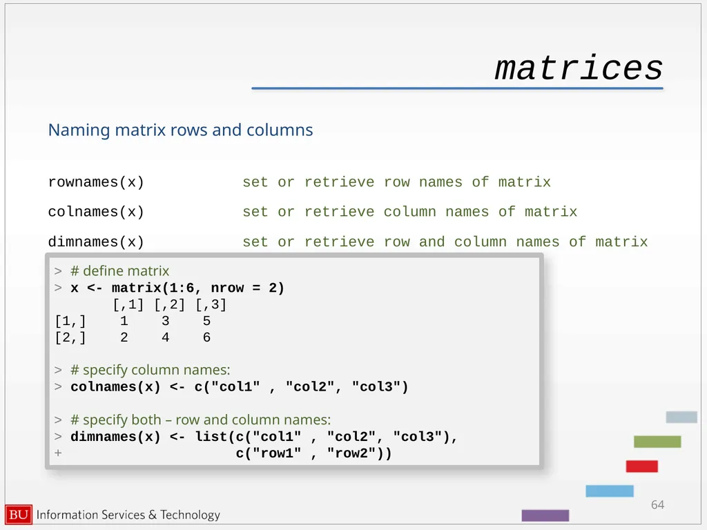
slide64. matrices 64 Naming matrix rows and columns

rownames(x) set or retrieve row names of matrix
colnames(x) set or retrieve column names of matrix
dimnames(x) set or retrieve row and column names of matrix > # define matrix
> x <- matrix(1:6, nrow = 2)
[,1] [,2] [,3]
[1,] 1 3 5
[2,] 2 4 6

> # specify column names:
> colnames(x) <- c("col1" , "col2", "col3")

> # specify both – row and column names:
> dimnames(x) <- list(c("col1" , "col2", "col3"),
+ c("row1" , "row2"))<br>
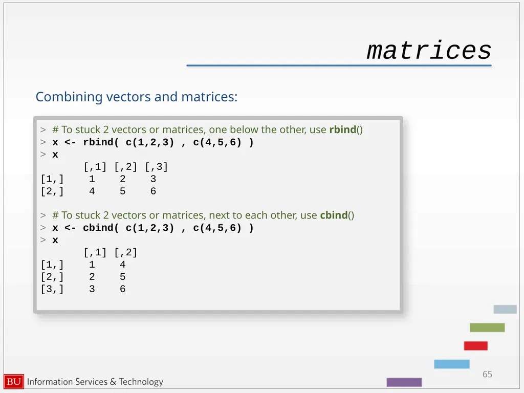
slide65. matrices 65 Combining vectors and matrices: > # To stuck 2 vectors or matrices, one below the other, use rbind()
> x <- rbind( c(1,2,3) , c(4,5,6) )
> x
[,1] [,2] [,3]
[1,] 1 2 3
[2,] 4 5 6

> # To stuck 2 vectors or matrices, next to each other, use cbind()
> x <- cbind( c(1,2,3) , c(4,5,6) )
> x
[,1] [,2]
[1,] 1 4
[2,] 2 5
[3,] 3 6<br>
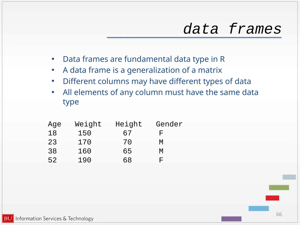
slide66. data frames Data frames are fundamental data type in R
A data frame is a generalization of a matrix
Different columns may have different types of data
All elements of any column must have the same data type 66 Age Weight Height Gender
18 150 67 F
23 170 70 M
38 160 65 M
52 190 68 F<br>
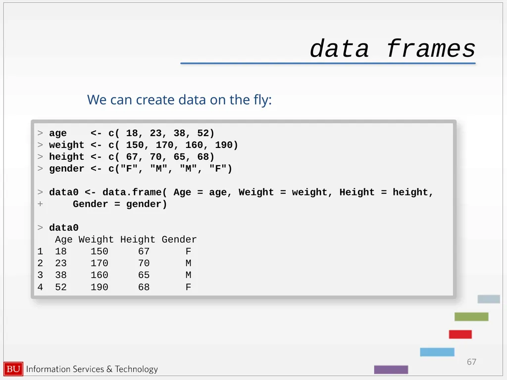
slide67. data frames We can create data on the fly: 67 > age <- c( 18, 23, 38, 52)
> weight <- c( 150, 170, 160, 190)
> height <- c( 67, 70, 65, 68)
> gender <- c("F", "M", "M", "F")

> data0 <- data.frame( Age = age, Weight = weight, Height = height,
+ Gender = gender)

> data0
Age Weight Height Gender
1 18 150 67 F
2 23 170 70 M
3 38 160 65 M
4 52 190 68 F<br>
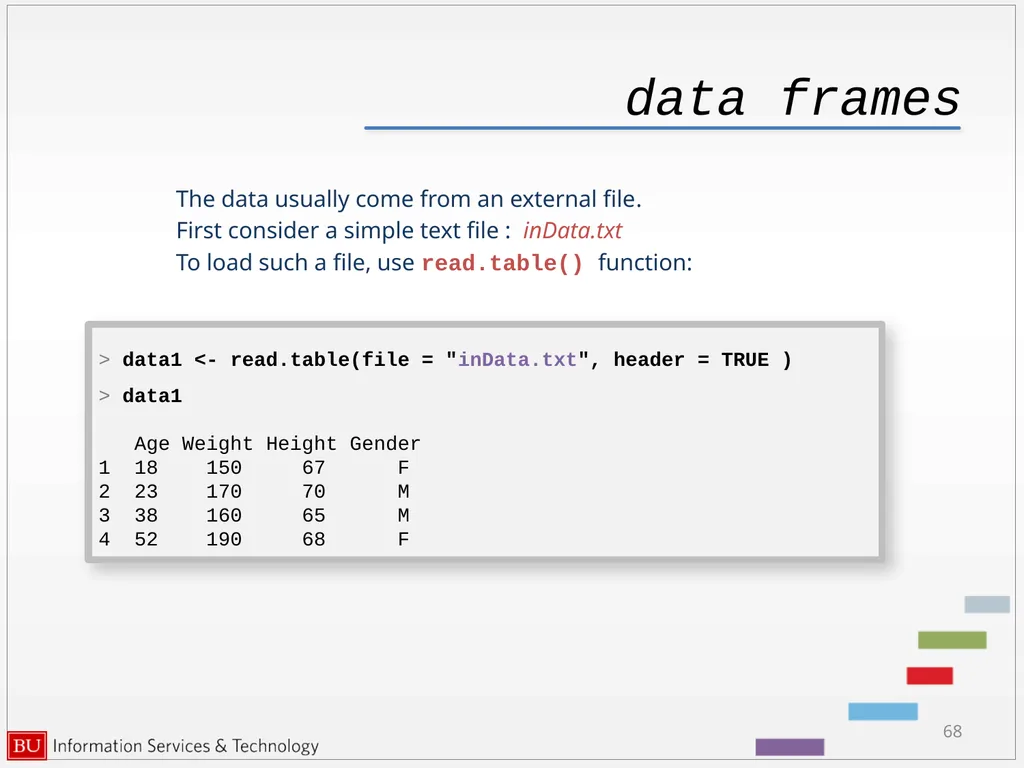
slide68. data frames The data usually come from an external file.
First consider a simple text file : inData.txt
To load such a file, use read.table() function: 68 > data1 <- read.table(file = "inData.txt", header = TRUE )
> data1

Age Weight Height Gender
1 18 150 67 F
2 23 170 70 M
3 38 160 65 M
4 52 190 68 F<br>
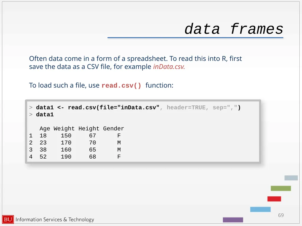
slide69. data frames Often data come in a form of a spreadsheet. To read this into R, first save the data as a CSV file, for example inData.csv.

To load such a file, use read.csv() function: 69 > data1 <- read.csv(file="inData.csv", header=TRUE, sep=",")
> data1

Age Weight Height Gender
1 18 150 67 F
2 23 170 70 M
3 38 160 65 M
4 52 190 68 F<br>
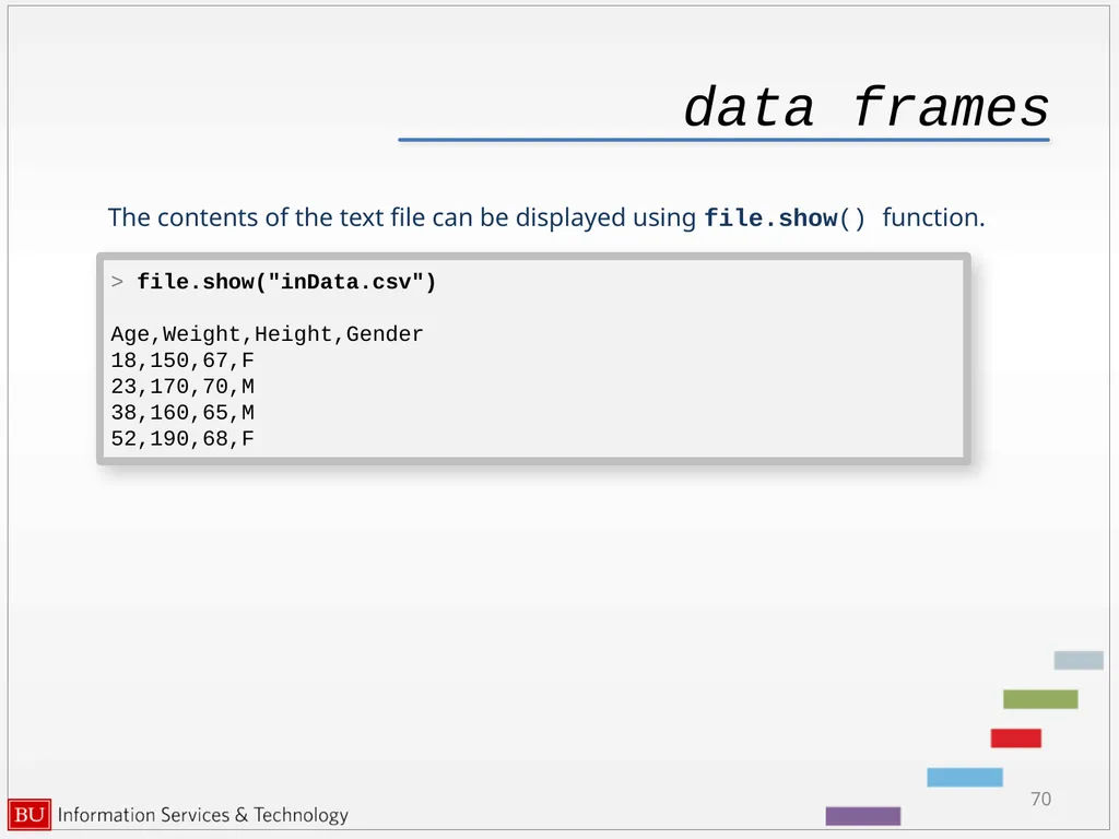
slide70. data frames The contents of the text file can be displayed using file.show() function. 70 > file.show("inData.csv")

Age,Weight,Height,Gender
18,150,67,F
23,170,70,M
38,160,65,M
52,190,68,F<br>
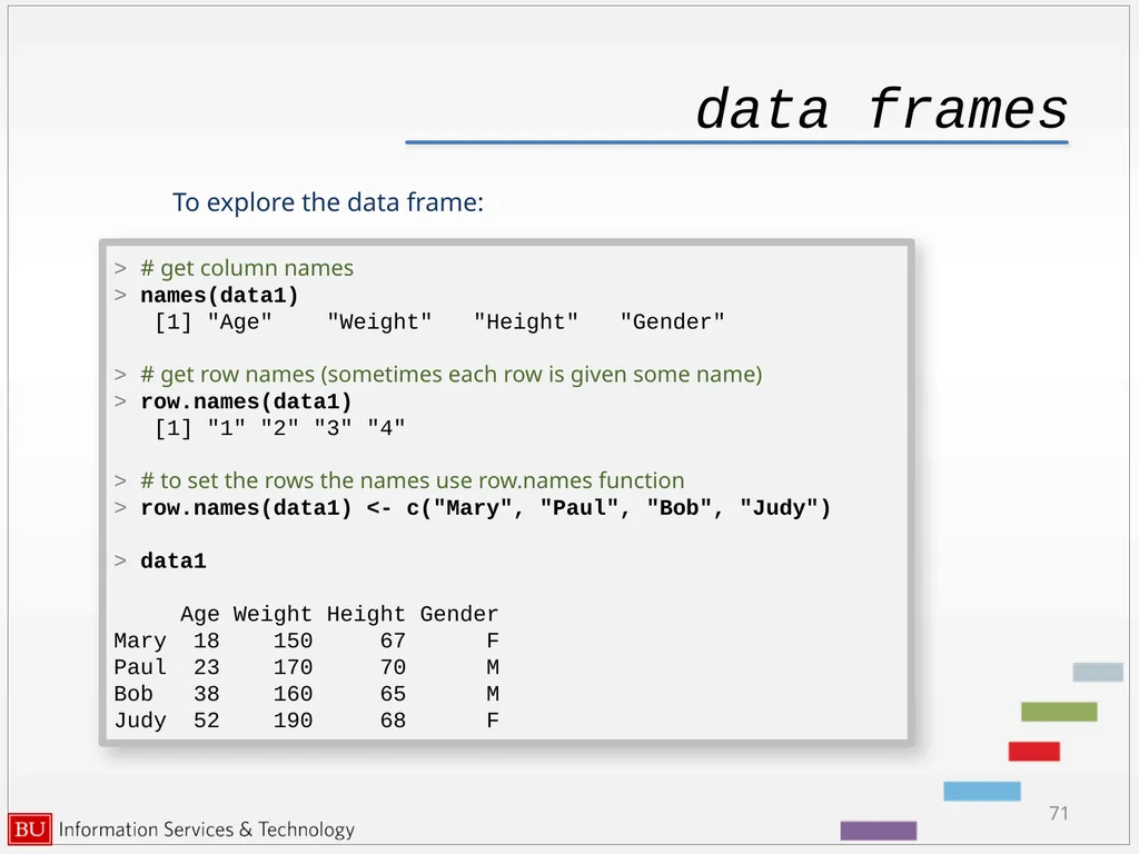
slide71. data frames To explore the data frame: 71 > # get column names
> names(data1)
[1] "Age" "Weight" "Height" "Gender"

> # get row names (sometimes each row is given some name)
> row.names(data1)
[1] "1" "2" "3" "4"

> # to set the rows the names use row.names function
> row.names(data1) <- c("Mary", "Paul", "Bob", "Judy")

> data1

Age Weight Height Gender
Mary 18 150 67 F
Paul 23 170 70 M
Bob 38 160 65 M
Judy 52 190 68 F<br>
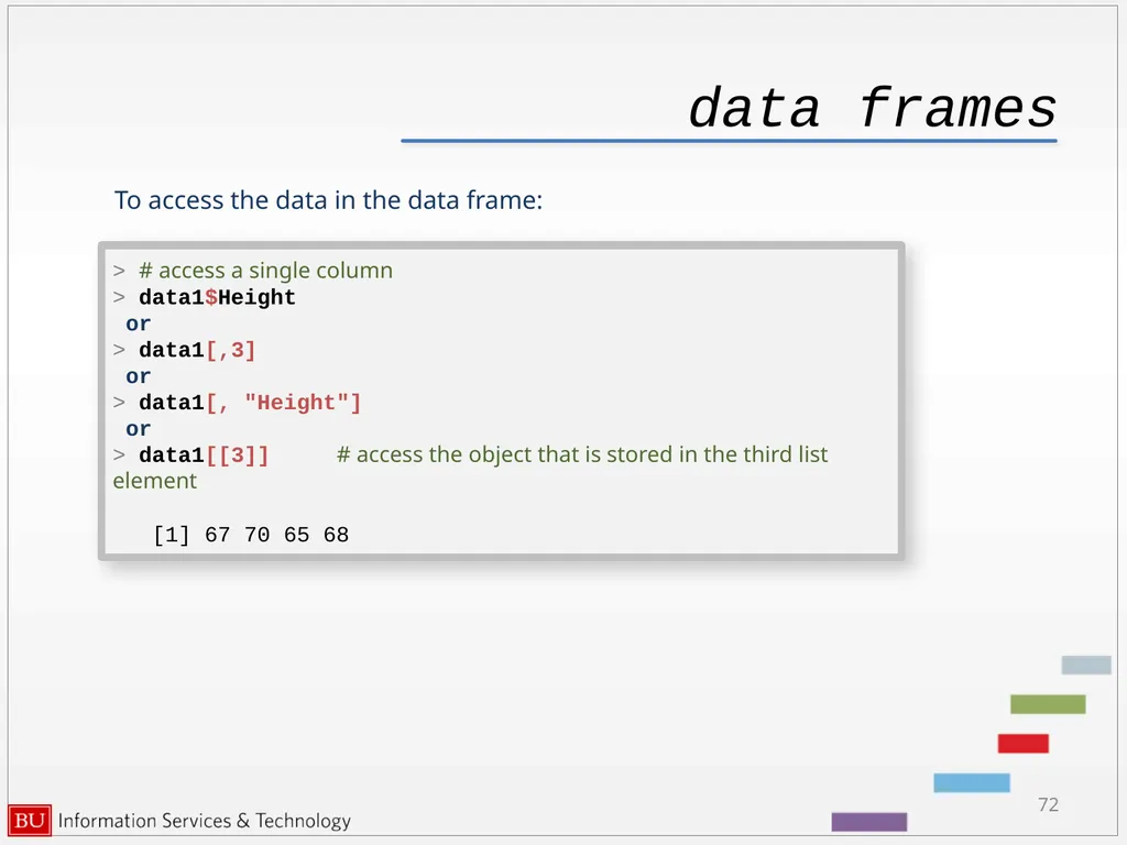
slide72. data frames 72 > # access a single column
> data1$Height
or
> data1[,3]
or
> data1[, "Height"]
or
> data1[[3]] # access the object that is stored in the third list element

[1] 67 70 65 68 To access the data in the data frame:<br>
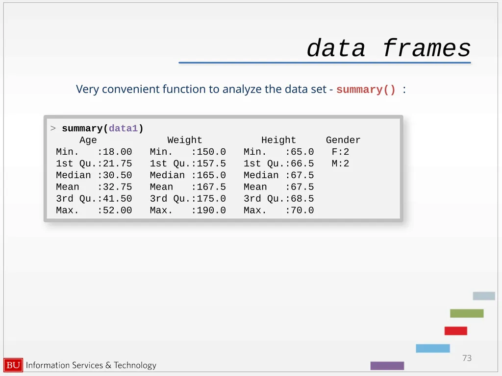
slide73. data frames Very convenient function to analyze the data set - summary() : 73 > summary(data1)
Age Weight Height Gender
Min. :18.00 Min. :150.0 Min. :65.0 F:2
1st Qu.:21.75 1st Qu.:157.5 1st Qu.:66.5 M:2
Median :30.50 Median :165.0 Median :67.5
Mean :32.75 Mean :167.5 Mean :67.5
3rd Qu.:41.50 3rd Qu.:175.0 3rd Qu.:68.5
Max. :52.00 Max. :190.0 Max. :70.0<br>
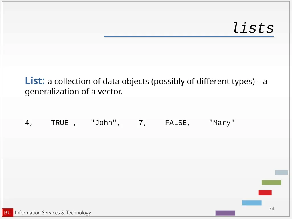
slide74. lists List: a collection of data objects (possibly of different types) – a generalization of a vector.

4, TRUE , "John", 7, FALSE, "Mary" 74<br>
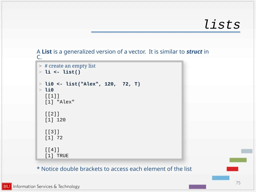
slide75. lists A List is a generalized version of a vector. It is similar to struct in C. 75 > # create an empty list
> li <- list()

> li0 <- list("Alex", 120, 72, T)
> li0
[[1]]
[1] "Alex"

[[2]]
[1] 120

[[3]]
[1] 72

[[4]]
[1] TRUE * Notice double brackets to access each element of the list<br>
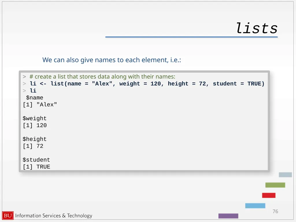
slide76. lists We can also give names to each element, i.e.: 76 > # create a list that stores data along with their names:
> li <- list(name = "Alex", weight = 120, height = 72, student = TRUE)
> li
$name
[1] "Alex"

$weight
[1] 120

$height
[1] 72

$student
[1] TRUE<br>
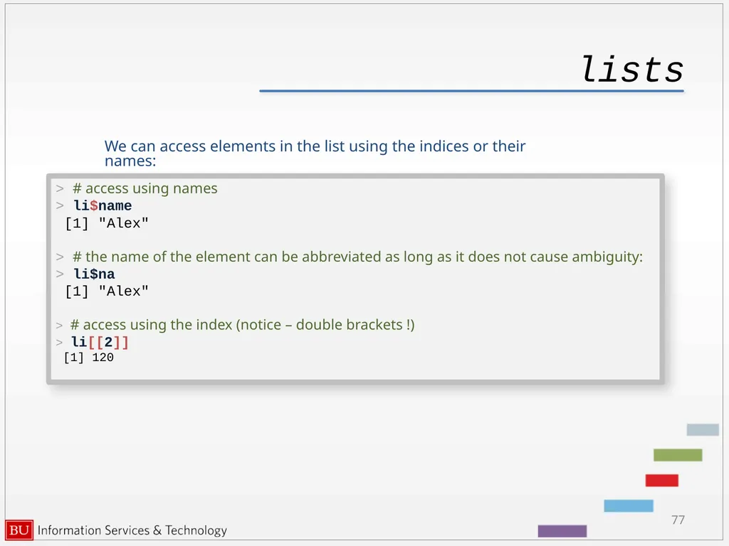
slide77. lists We can access elements in the list using the indices or their names: 77 > # access using names
> li$name
[1] "Alex"

> # the name of the element can be abbreviated as long as it does not cause ambiguity:
> li$na
[1] "Alex"

> # access using the index (notice – double brackets !)
> li[[2]]
[1] 120<br>
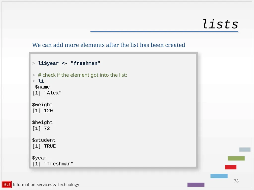
slide78. lists We can add more elements after the list has been created 78 > li$year <- "freshman"

> # check if the element got into the list:
> li
$name
[1] "Alex"

$weight
[1] 120

$height
[1] 72

$student
[1] TRUE

$year
[1] "freshman"<br>
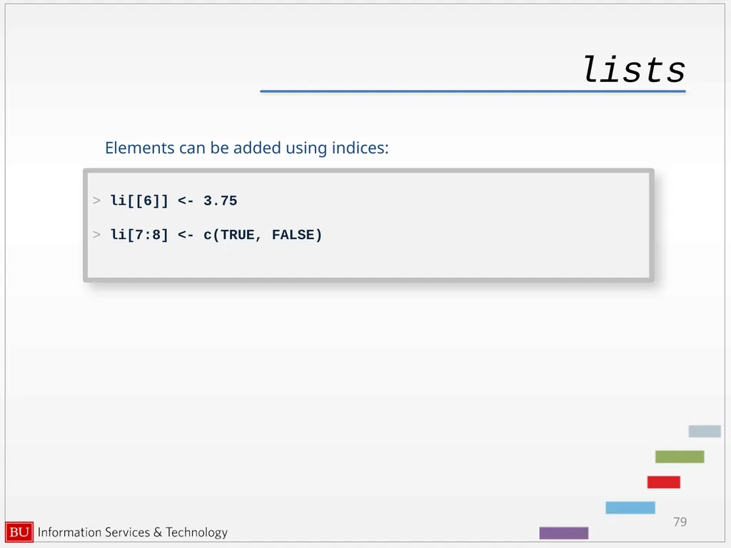
slide79. lists Elements can be added using indices: 79 > li[[6]] <- 3.75

> li[7:8] <- c(TRUE, FALSE)<br>
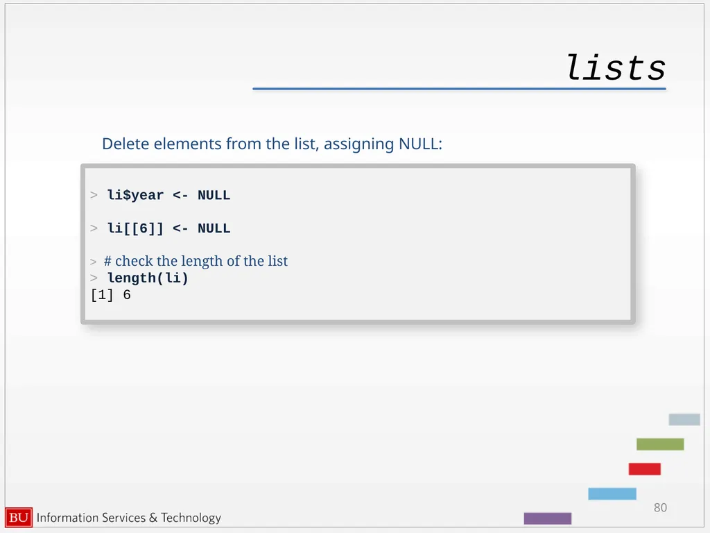
slide80. lists Delete elements from the list, assigning NULL: 80 > li$year <- NULL

> li[[6]] <- NULL

> # check the length of the list
> length(li)
[1] 6<br>
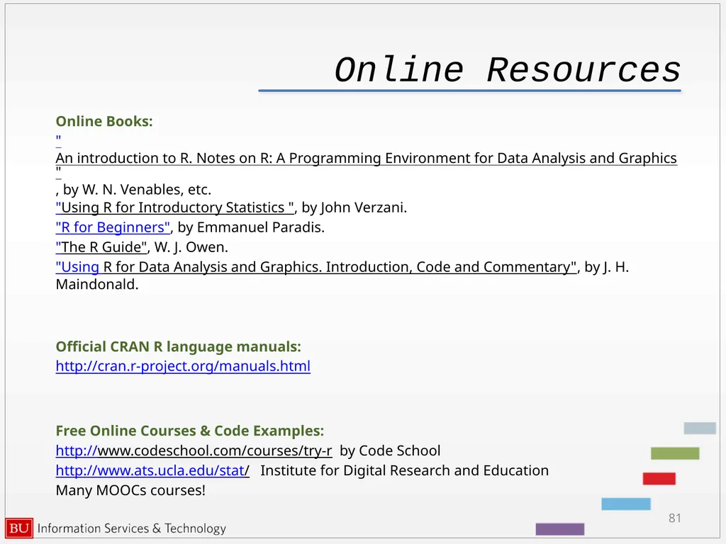
slide81. Online Resources Online Books:
"An introduction to R. Notes on R: A Programming Environment for Data Analysis and Graphics", by W. N. Venables, etc.
"Using R for Introductory Statistics ", by John Verzani.
"R for Beginners", by Emmanuel Paradis.
"The R Guide", W. J. Owen.
"Using R for Data Analysis and Graphics. Introduction, Code and Commentary", by J. H. Maindonald.

Official CRAN R language manuals:
http://cran.r-project.org/manuals.html

Free Online Courses & Code Examples:
http://www.codeschool.com/courses/try-r by Code School
http://www.ats.ucla.edu/stat/ Institute for Digital Research and Education
Many MOOCs courses! 81<br>
slide82. 82 This tutorial has been made possible by
Scientific Computing and Visualization
group
at Boston University.

Katia Oleinikkoleinik@bu.edu

http://www.bu.edu/tech/research/training/tutorials/list/<br>