Knowledge Tracing Week 9 Goal of Knowledge Tracing

slide1. Knowledge Tracing Week 9<br>
slide2. Goal of Knowledge Tracing Measuring what a student knows at a specific time

Measuring what relevant knowledge components a student knows at a specific time<br>
slide3. Knowledge Component Anything a student can know that is meaningful to the current learning situation

Skill
Fact
Concept
Principle
Schema

http://www.learnlab.org/research/wiki/index.php/Knowledge_component<br>
slide4. Why is it useful to measure student knowledge? Enhancing student knowledge is the primary goal of a lot of education
If you can measure it, you know whether you’re making it better
If you can measure it, you can inform instructors (and other stakeholders) about it
If you can measure it, you can make automated pedagogical decisions<br>
slide5. Different than measuring performance Inferring if a student’s performance right now is associated with successfully demonstrating a skill

Not the same as knowing whether the student has a skill, which is not directly observable
Maybe they appeared to demonstrate skill without having it (“guess”)
Maybe they appeared to not demonstrate skill despite having it (“slip”)<br>
slide6. How do we get at latent knowledge? We can’t measure it directly
We can’t look directly into the brain
Yet

But we can look at performance
And we can look at performance over time
More information than performance at one specific moment<br>
slide7. Not trivial… This is a research problem with a long history…<br>
slide8. This week I will cover some of the key approaches for knowledge tracing, within EDM<br>
slide9. First Up Bayesian Knowledge Tracing<br>
slide10. Bayesian Knowledge Tracing (BKT) The classic approach for measuring tightly defined skill in online learning

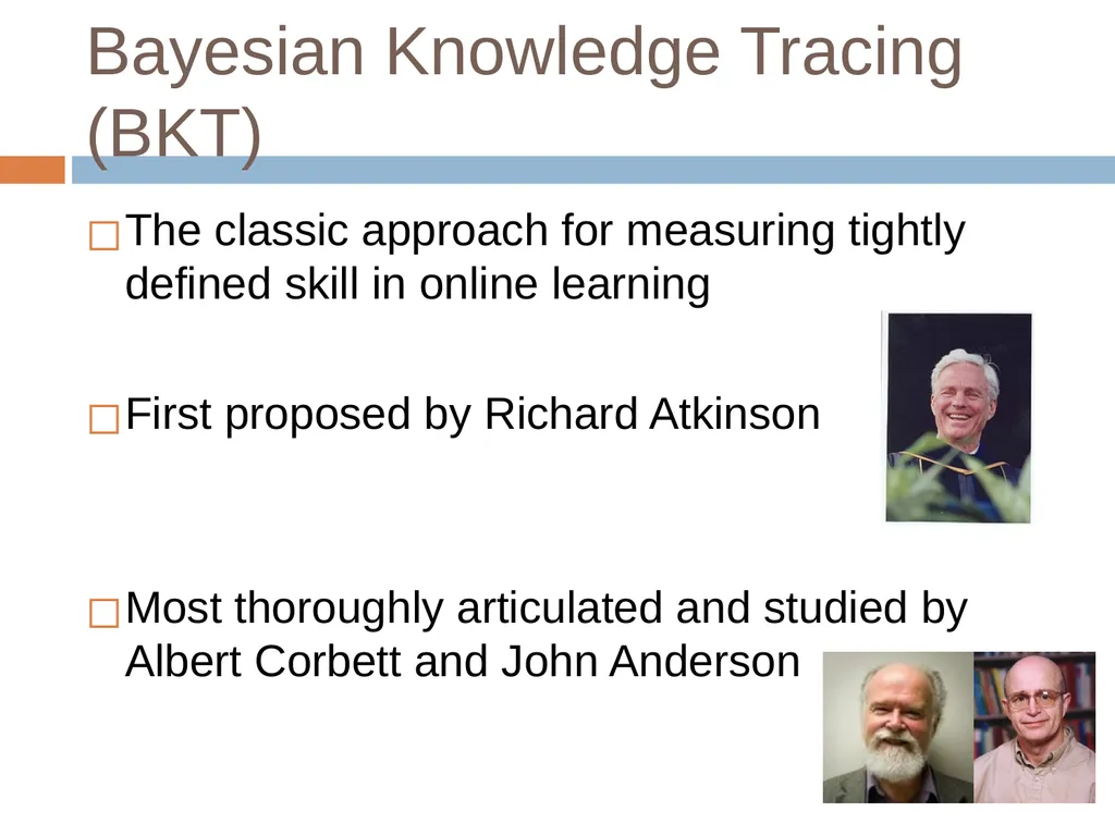
First proposed by Richard Atkinson

Most thoroughly articulated and studied by Albert Corbett and John Anderson<br>
slide11. Bayesian Knowledge Tracing (BKT) Been around a long time

Still (as of this recording, Fall 2023) the most widely-used knowledge tracing algorithm used at scale
Interpretable
Predictable
Decent performance<br>
slide12. The key goal of BKT Measuring how well a student knows a specific skill/knowledge component at a specific time

Based on their past history of performance with that skill/KC<br>
slide13. Skills should be tightly defined Unlike approaches such as Item Response Theory (later this week)

The goal is not to measure overall skill for a broadly-defined construct
Such as arithmetic

But to measure a specific skill or knowledge component
Such as addition of two-digit numbers where no carrying is needed<br>
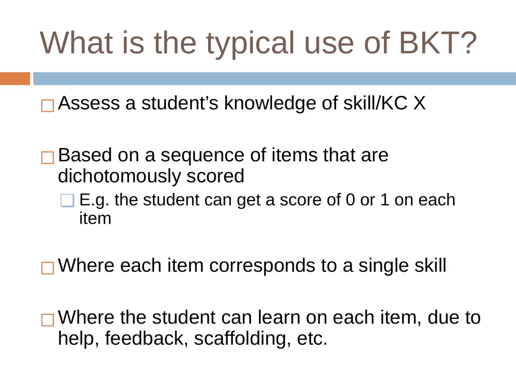
slide14. What is the typical use of BKT? Assess a student’s knowledge of skill/KC X

Based on a sequence of items that are dichotomously scored
E.g. the student can get a score of 0 or 1 on each item

Where each item corresponds to a single skill

Where the student can learn on each item, due to help, feedback, scaffolding, etc.<br>
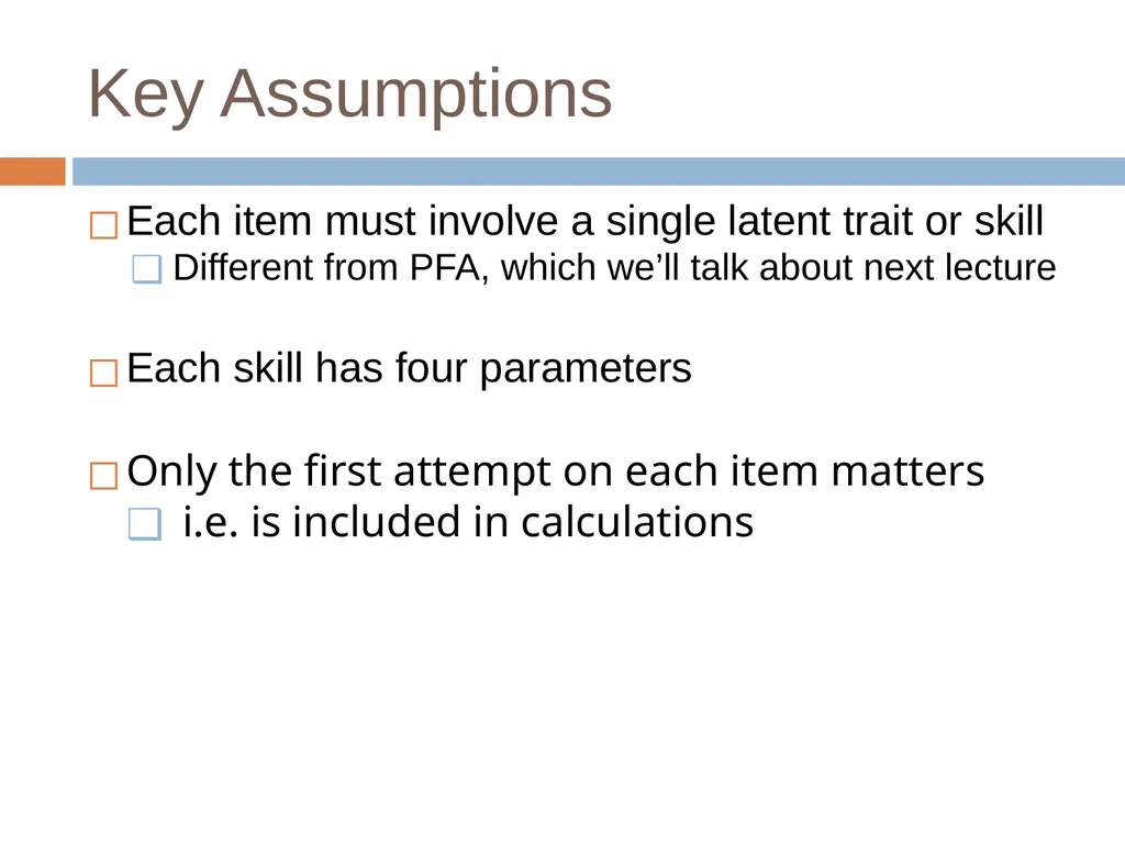
slide15. Key Assumptions Each item must involve a single latent trait or skill
Different from PFA, which we’ll talk about next lecture

Each skill has four parameters

Only the first attempt on each item matters
i.e. is included in calculations<br>
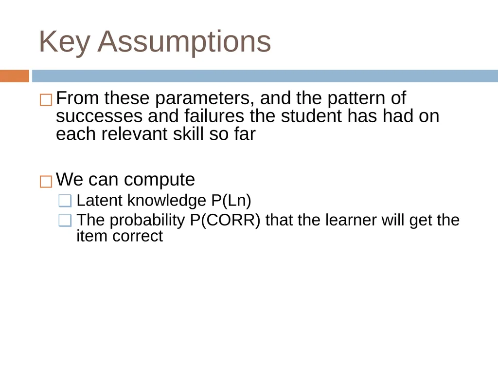
slide16. Key Assumptions From these parameters, and the pattern of successes and failures the student has had on each relevant skill so far

We can compute
Latent knowledge P(Ln)
The probability P(CORR) that the learner will get the item correct<br>
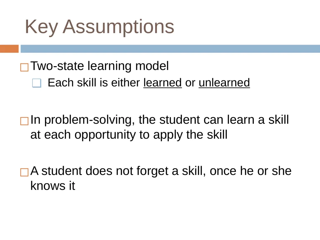
slide17. Key Assumptions Two-state learning model
Each skill is either learned or unlearned

In problem-solving, the student can learn a skill at each opportunity to apply the skill

A student does not forget a skill, once he or she knows it<br>
slide18. Model Performance Assumptions If the student knows a skill, there is still some chance the student will slip and make a mistake.

If the student does not know a skill, there is still some chance the student will guess correctly.<br>
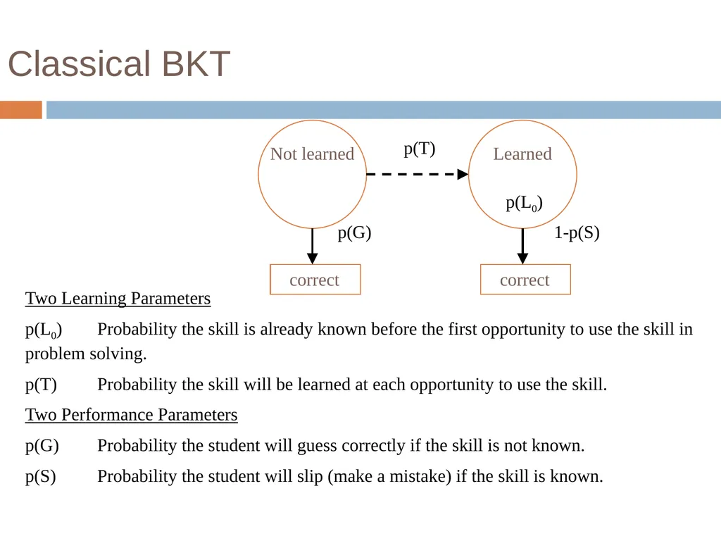
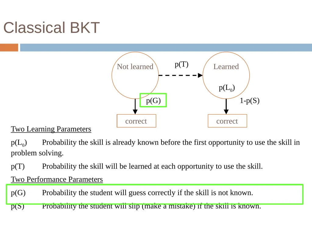
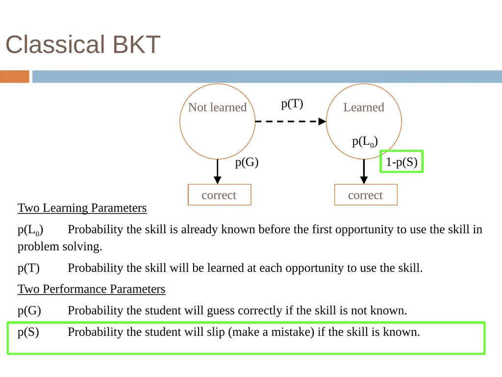
slide19. Classical BKT Not learned Two Learning Parameters
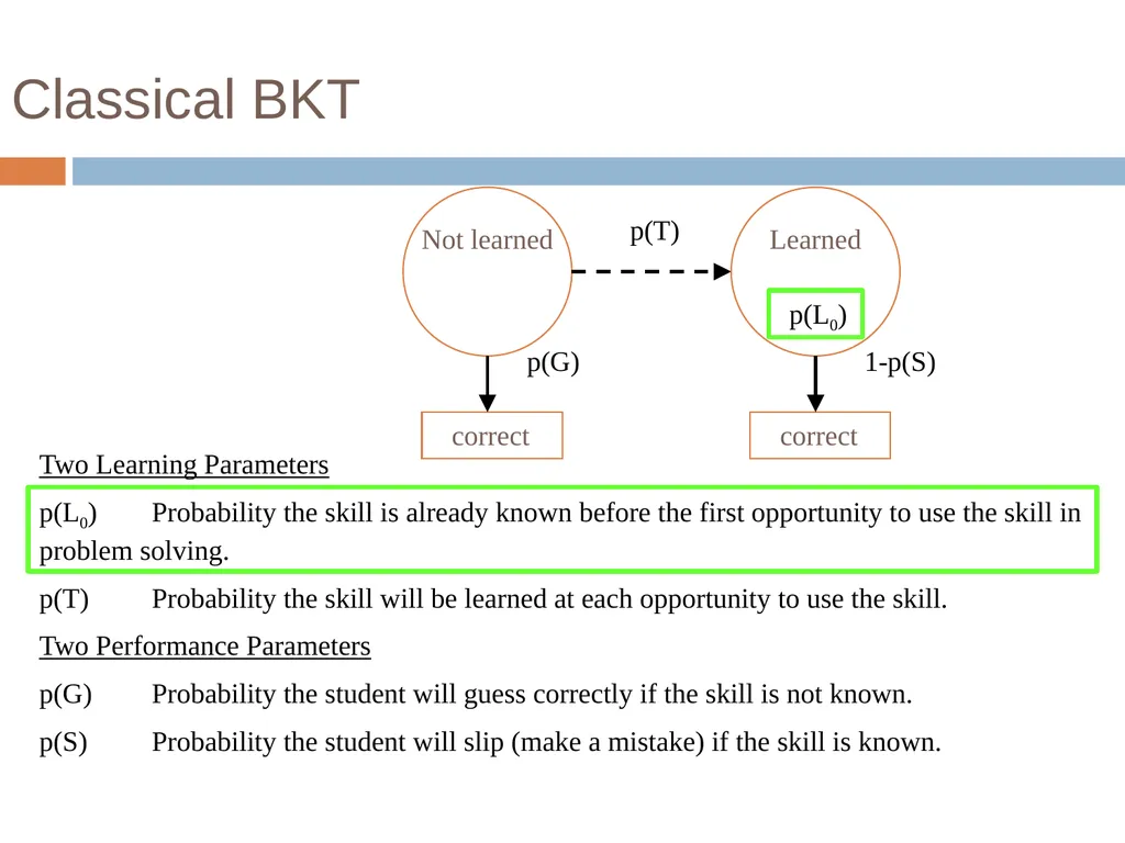
p(L0) Probability the skill is already known before the first opportunity to use the skill in problem solving.
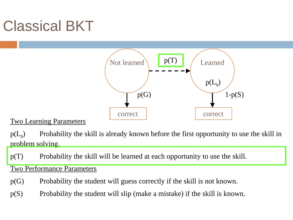
p(T) Probability the skill will be learned at each opportunity to use the skill.
Two Performance Parameters
p(G) Probability the student will guess correctly if the skill is not known.
p(S) Probability the student will slip (make a mistake) if the skill is known. Learned p(T) correct correct p(G) 1-p(S) p(L0)<br>
slide20. Classical BKT Not learned Two Learning Parameters
p(L0) Probability the skill is already known before the first opportunity to use the skill in problem solving.
p(T) Probability the skill will be learned at each opportunity to use the skill.
Two Performance Parameters
p(G) Probability the student will guess correctly if the skill is not known.
p(S) Probability the student will slip (make a mistake) if the skill is known. Learned p(T) correct correct p(G) 1-p(S) p(L0)<br>
slide21. Classical BKT Not learned Two Learning Parameters
p(L0) Probability the skill is already known before the first opportunity to use the skill in problem solving.
p(T) Probability the skill will be learned at each opportunity to use the skill.
Two Performance Parameters
p(G) Probability the student will guess correctly if the skill is not known.
p(S) Probability the student will slip (make a mistake) if the skill is known. Learned p(T) correct correct p(G) 1-p(S) p(L0)<br>
slide22. Classical BKT Not learned Two Learning Parameters
p(L0) Probability the skill is already known before the first opportunity to use the skill in problem solving.
p(T) Probability the skill will be learned at each opportunity to use the skill.
Two Performance Parameters
p(G) Probability the student will guess correctly if the skill is not known.
p(S) Probability the student will slip (make a mistake) if the skill is known. Learned p(T) correct correct p(G) 1-p(S) p(L0)<br>
slide23. Classical BKT Not learned Two Learning Parameters
p(L0) Probability the skill is already known before the first opportunity to use the skill in problem solving.
p(T) Probability the skill will be learned at each opportunity to use the skill.
Two Performance Parameters
p(G) Probability the student will guess correctly if the skill is not known.
p(S) Probability the student will slip (make a mistake) if the skill is known. Learned p(T) correct correct p(G) 1-p(S) p(L0)<br>
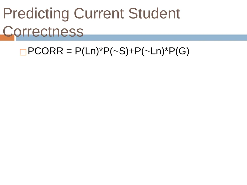
slide24. Predicting Current Student Correctness PCORR = P(Ln)*P(~S)+P(~Ln)*P(G)<br>
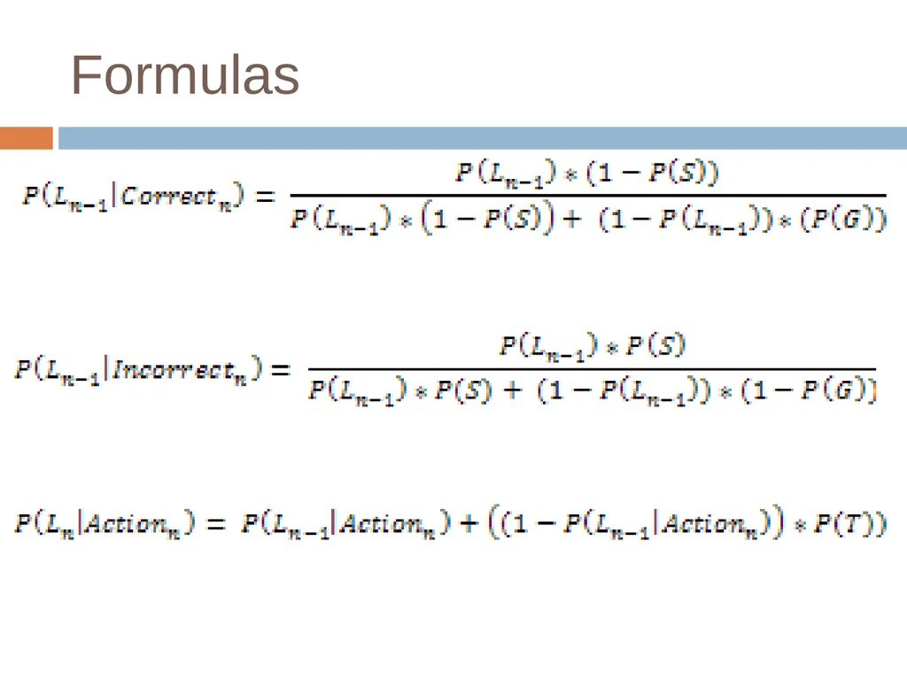
slide25. Bayesian Knowledge Tracing Whenever the student has an opportunity to use a skill

The probability that the student knows the skill is updated

Using formulas derived from Bayes’ Theorem.<br>
slide26. Formulas<br>
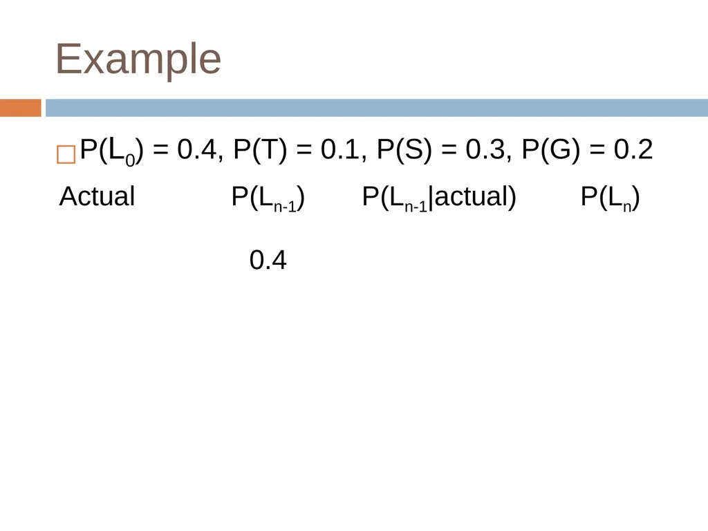
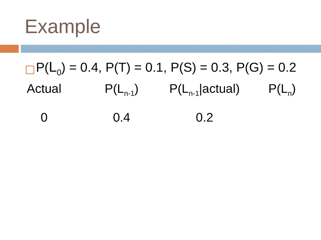
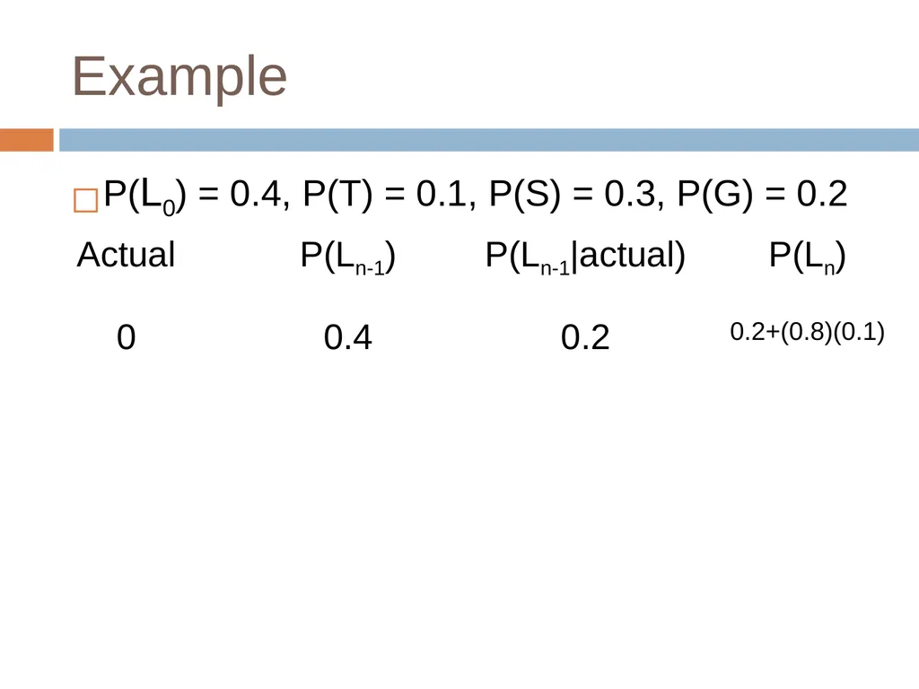
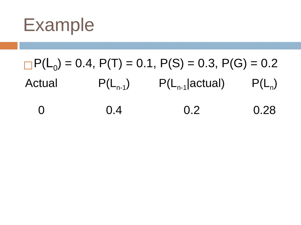
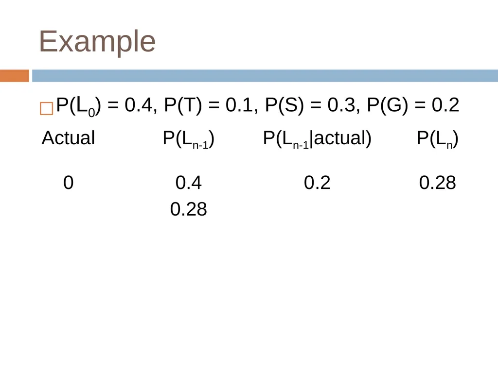
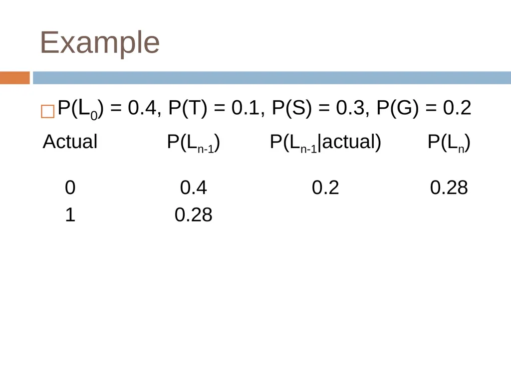
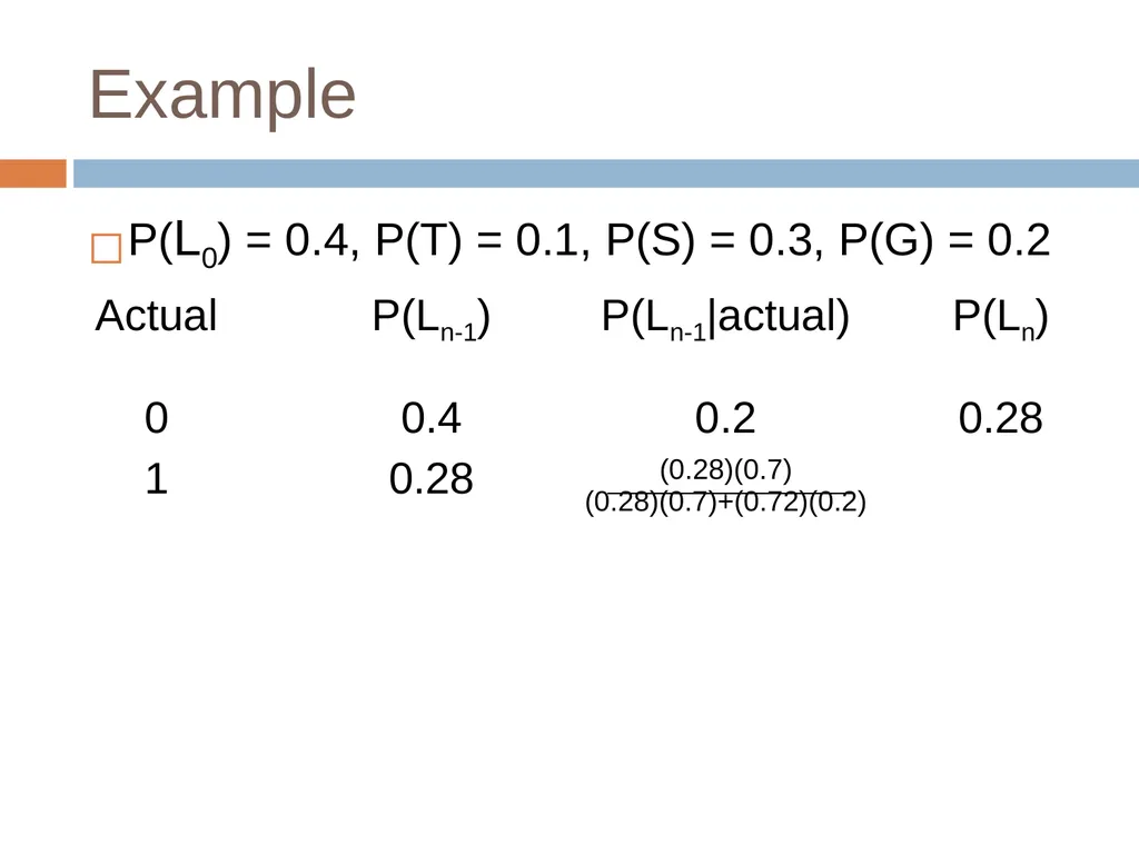
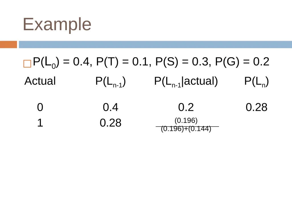
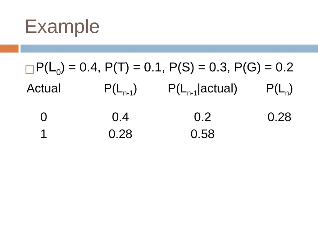
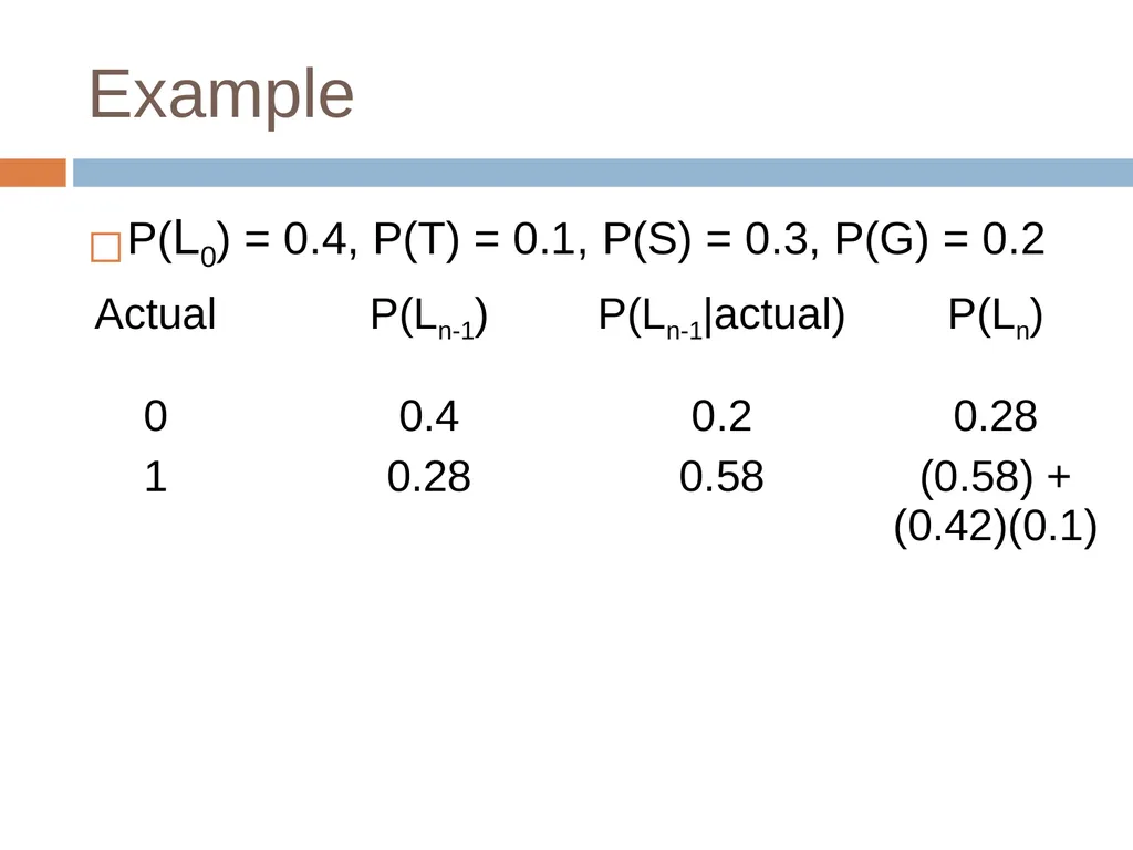
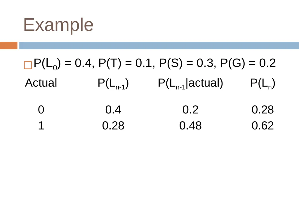
slide27. Example P(L0) = 0.4, P(T) = 0.1, P(S) = 0.3, P(G) = 0.2<br>
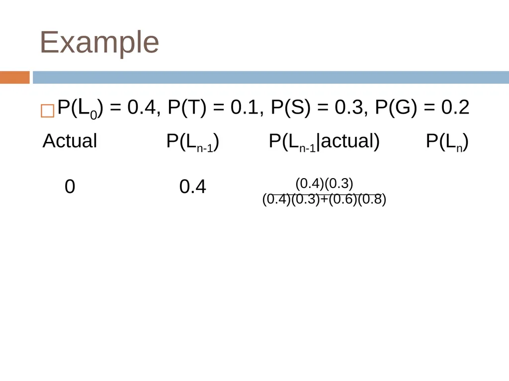
slide28. Example P(L0) = 0.4, P(T) = 0.1, P(S) = 0.3, P(G) = 0.2<br>
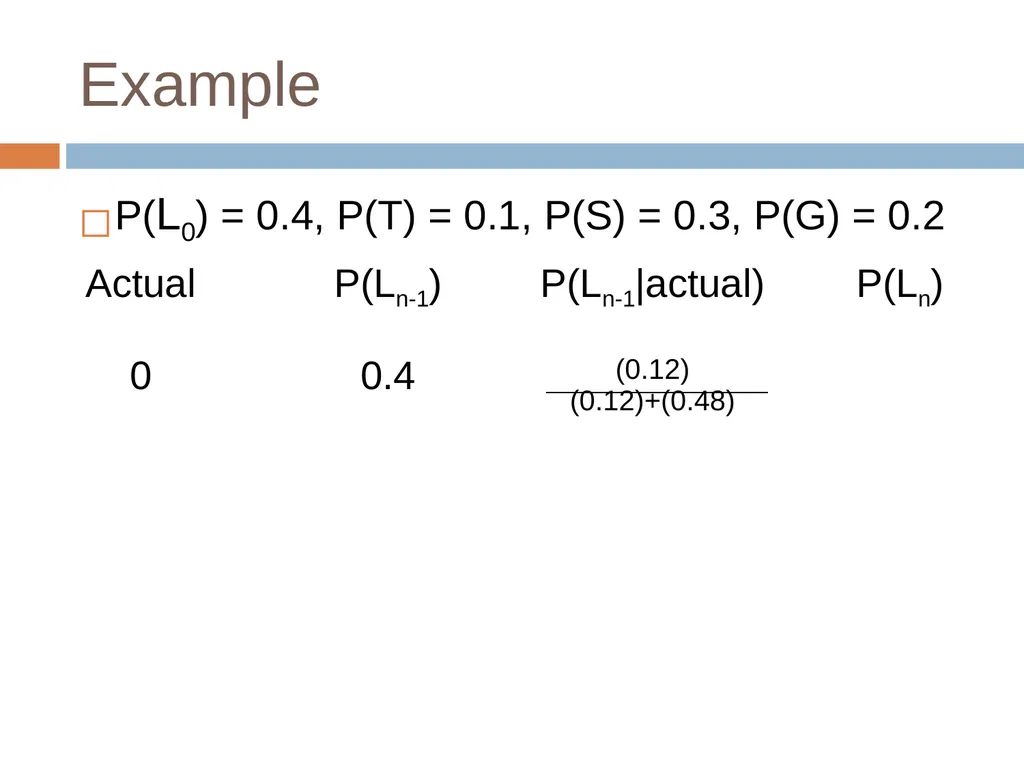
slide29. Example P(L0) = 0.4, P(T) = 0.1, P(S) = 0.3, P(G) = 0.2<br>
slide30. Example P(L0) = 0.4, P(T) = 0.1, P(S) = 0.3, P(G) = 0.2<br>
slide31. Example P(L0) = 0.4, P(T) = 0.1, P(S) = 0.3, P(G) = 0.2<br>
slide32. Example P(L0) = 0.4, P(T) = 0.1, P(S) = 0.3, P(G) = 0.2<br>
slide33. Example P(L0) = 0.4, P(T) = 0.1, P(S) = 0.3, P(G) = 0.2<br>
slide34. Example P(L0) = 0.4, P(T) = 0.1, P(S) = 0.3, P(G) = 0.2<br>
slide35. Example P(L0) = 0.4, P(T) = 0.1, P(S) = 0.3, P(G) = 0.2<br>
slide36. Example P(L0) = 0.4, P(T) = 0.1, P(S) = 0.3, P(G) = 0.2<br>
slide37. Example P(L0) = 0.4, P(T) = 0.1, P(S) = 0.3, P(G) = 0.2<br>
slide38. Example P(L0) = 0.4, P(T) = 0.1, P(S) = 0.3, P(G) = 0.2<br>
slide39. Example P(L0) = 0.4, P(T) = 0.1, P(S) = 0.3, P(G) = 0.2<br>
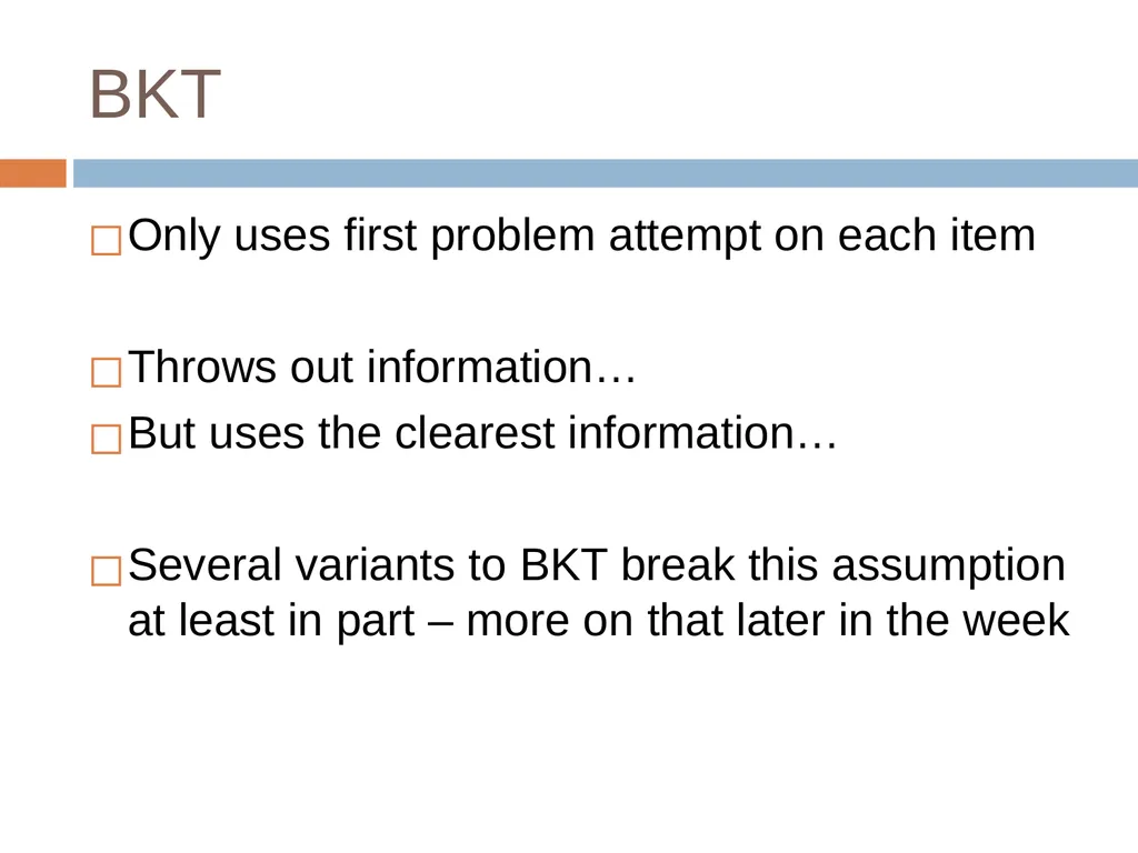
slide40. BKT Only uses first problem attempt on each item

Throws out information…
But uses the clearest information…

Several variants to BKT break this assumption at least in part – more on that later in the week<br>
slide41. Parameter Constraints Typically, the potential values of BKT parameters are constrained
To avoid model degeneracy<br>
slide42. Conceptual Idea Behind Knowledge Tracing Knowing a skill generally leads to correct performance
Correct performance implies that a student knows the relevant skill

Hence, by looking at whether a student’s performance is correct, we can infer whether they know the skill<br>
slide43. Essentially A knowledge model is degenerate when it violates this idea

When knowing a skill leads to worse performance

When getting a skill wrong means you know it<br>
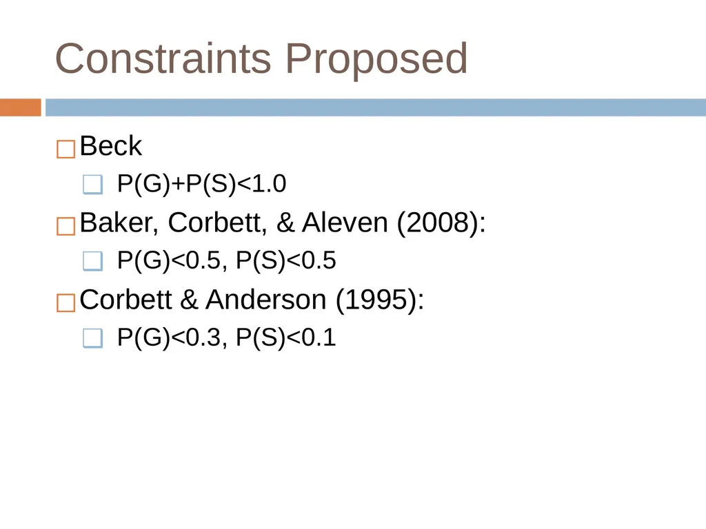
slide44. Constraints Proposed Beck
P(G)+P(S)<1.0
Baker, Corbett, & Aleven (2008):
P(G)<0.5, P(S)<0.5
Corbett & Anderson (1995):
P(G)<0.3, P(S)<0.1<br>
slide45. Knowledge Tracing How do we know if a knowledge tracing model is any good?

Our primary goal is to predict knowledge<br>
slide46. Knowledge Tracing How do we know if a knowledge tracing model is any good?

Our primary goal is to predict knowledge

But knowledge is a latent trait<br>
slide47. Knowledge Tracing How do we know if a knowledge tracing model is any good?

Our primary goal is to predict knowledge

But knowledge is latent

So we instead check our knowledge predictions by checking how well the model predicts performance<br>
slide48. Fitting a Knowledge-Tracing Model In principle, any set of four parameters can be used by knowledge-tracing

But parameters that predict student performance better are preferred<br>
slide49. Knowledge Tracing So, we pick the knowledge tracing parameters that best predict performance

Defined as whether a student’s action will be correct or wrong at a given time<br>
slide50. Fit Methods I could spend an hour talking about the ways to fit Bayesian Knowledge Tracing models<br>
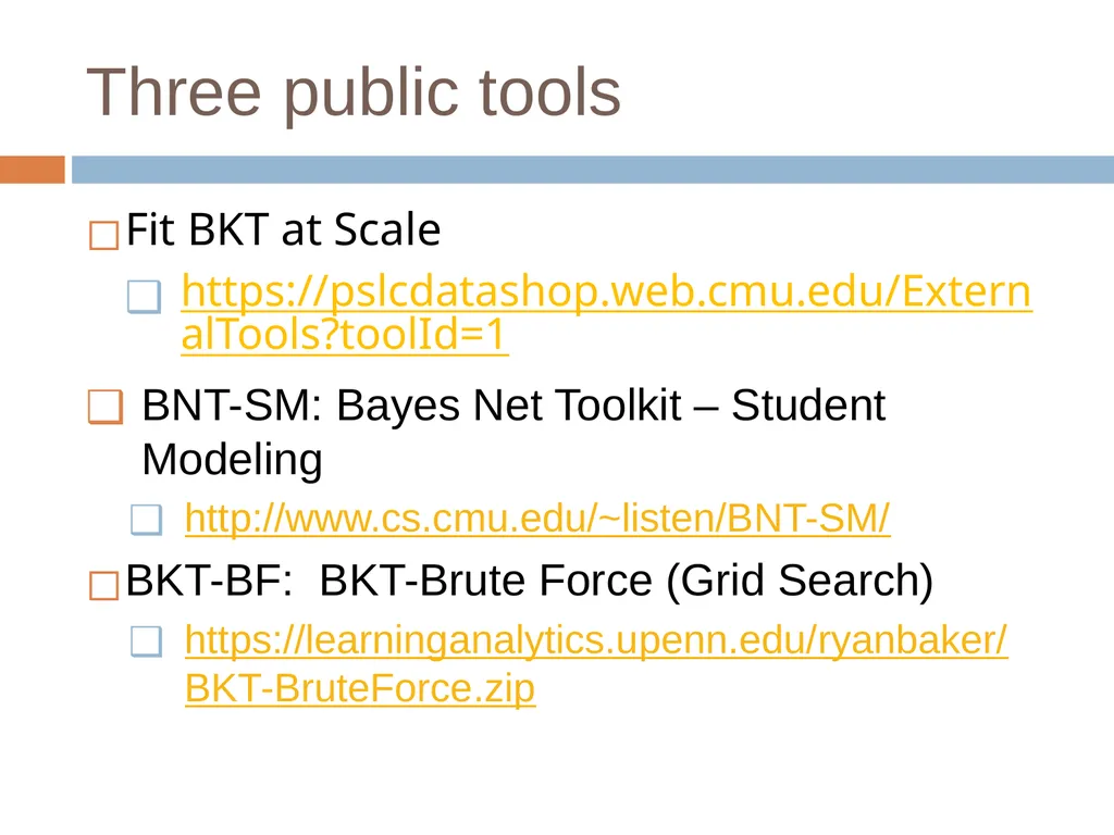
slide51. Three public tools Fit BKT at Scale
https://pslcdatashop.web.cmu.edu/ExternalTools?toolId=1
BNT-SM: Bayes Net Toolkit – Student Modeling
http://www.cs.cmu.edu/~listen/BNT-SM/
BKT-BF: BKT-Brute Force (Grid Search)
https://learninganalytics.upenn.edu/ryanbaker/BKT-BruteForce.zip<br>
slide52. Which one should you use? They’re all fine – they work approximately equally well

My group uses BKT-BF to fit Classical BKT and BNT-SM to fit variant models
But some commercial colleagues use Fit BKT at Scale<br>
slide53. Note… The Equation Solver in Excel replicably does worse for this problem than these packages<br>
slide54. Extensions There have been many extensions to BKT

We will discuss some of the most important ones in class, later in the week<br>
slide55. Sample Size There is a way to determine how big a sample size you need for BKT
Depends both on number of students and number of practices per student
This is not currently available for any other knowledge tracing algorithm (that assesses knowledge as it changes)

(Slater & Baker, Behaviormetrika, 2018)<br>
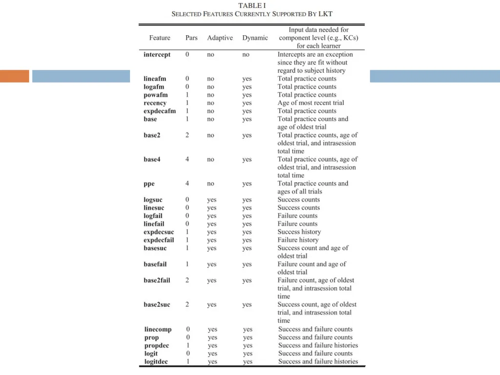
slide56. Logistic Knowledge Tracing A broad framework for knowledge tracing models based on logistic regression (Pavlik et al., 2021)<br>
slide57. Performance Factors Analysis First member of the LKT family that ran in real-time(Pavlik et al., 2009)<br>
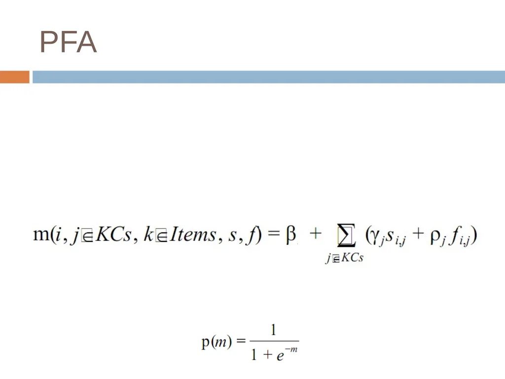
slide58. PFA Measures how much latent skill a student has, while they are learning
But expresses it in terms of probability of correctness, the next time the skill is encountered
No direct expression of the amount of latent skill, except this probability of correctness<br>
slide59. What is the typical use of PFA? Assess a student’s knowledge of topic X

Based on a sequence of items that are dichotomously scored
E.g. the student can get a score of 0 or 1 on each item

Where the student can learn on each item, due to help, feedback, scaffolding, etc.<br>
slide60. How does PFA differ from BKT?<br>
slide61. Key assumptions Each item may involve multiple latent skills or knowledge components
Different from BKT

Each skill has success learning rate γ and failure learning rate ρ
Different from BKT where learning rate is the same, success or failure<br>
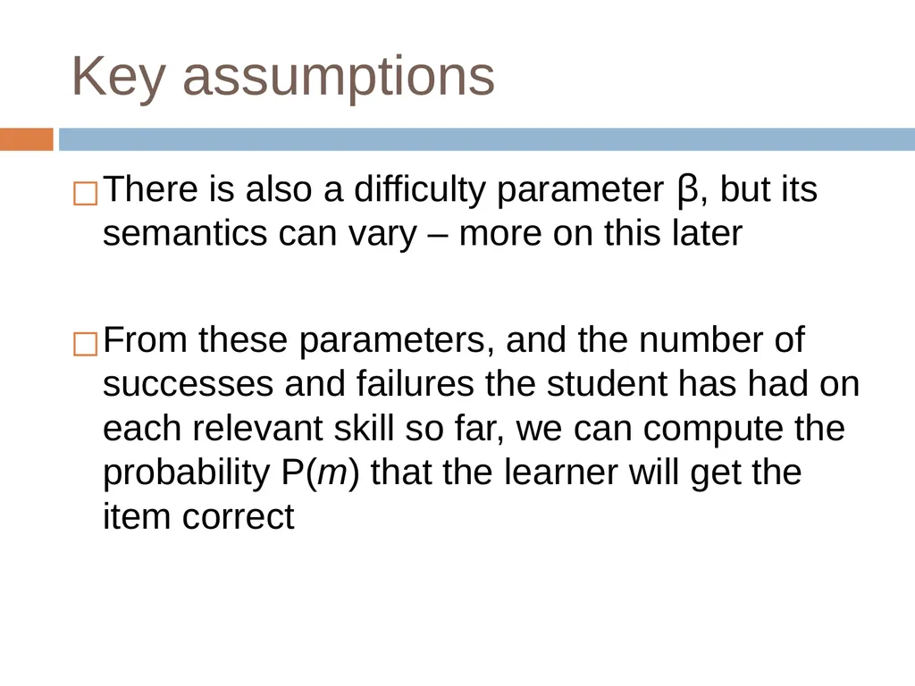
slide62. Key assumptions There is also a difficulty parameter β, but its semantics can vary – more on this later

From these parameters, and the number of successes and failures the student has had on each relevant skill so far, we can compute the probability P(m) that the learner will get the item correct<br>
slide63. PFA<br>
slide64. PFA<br>
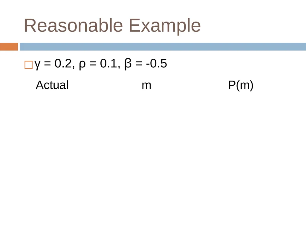
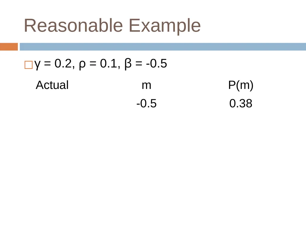
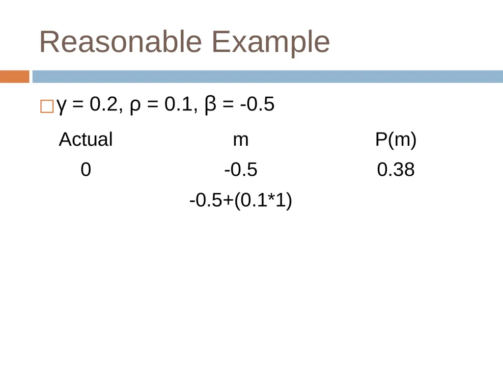
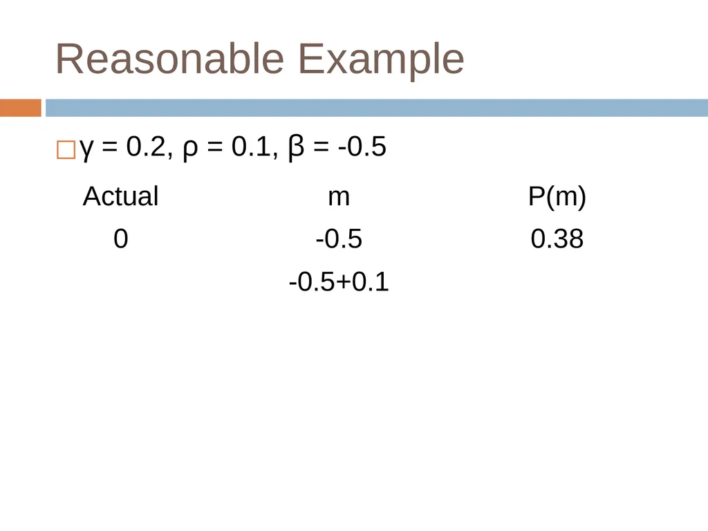
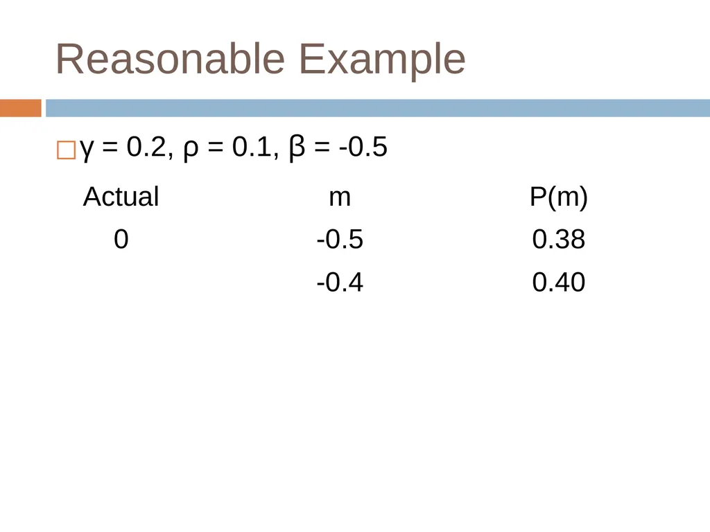
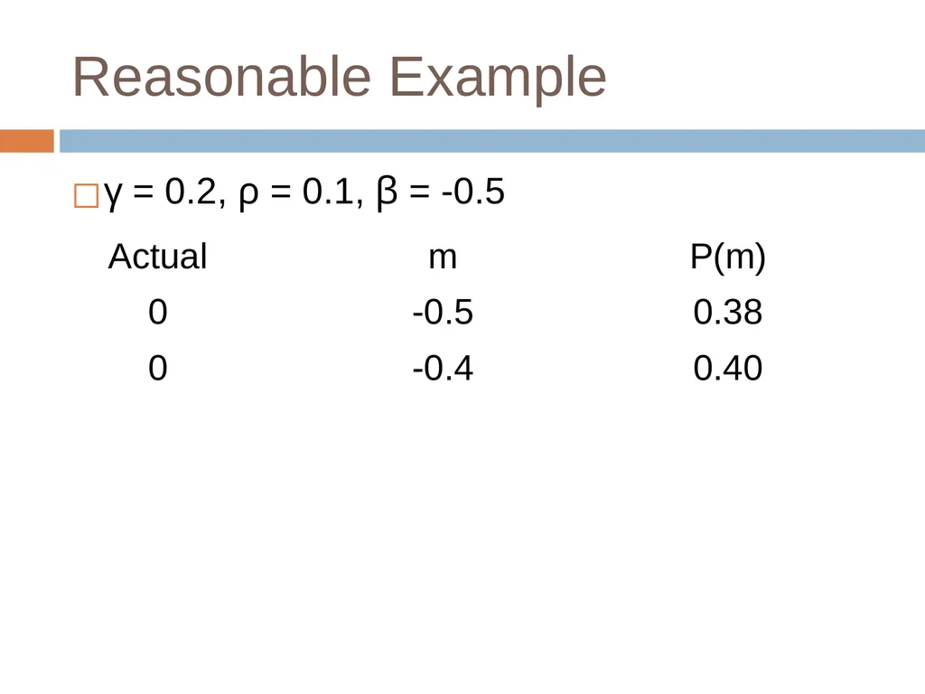
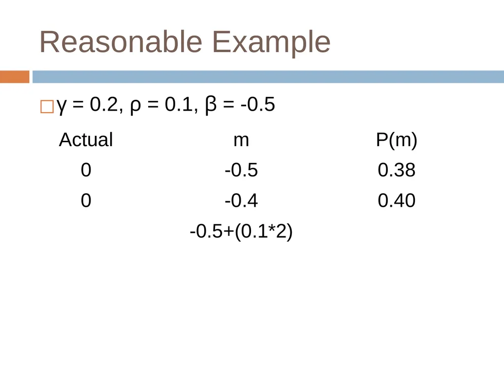
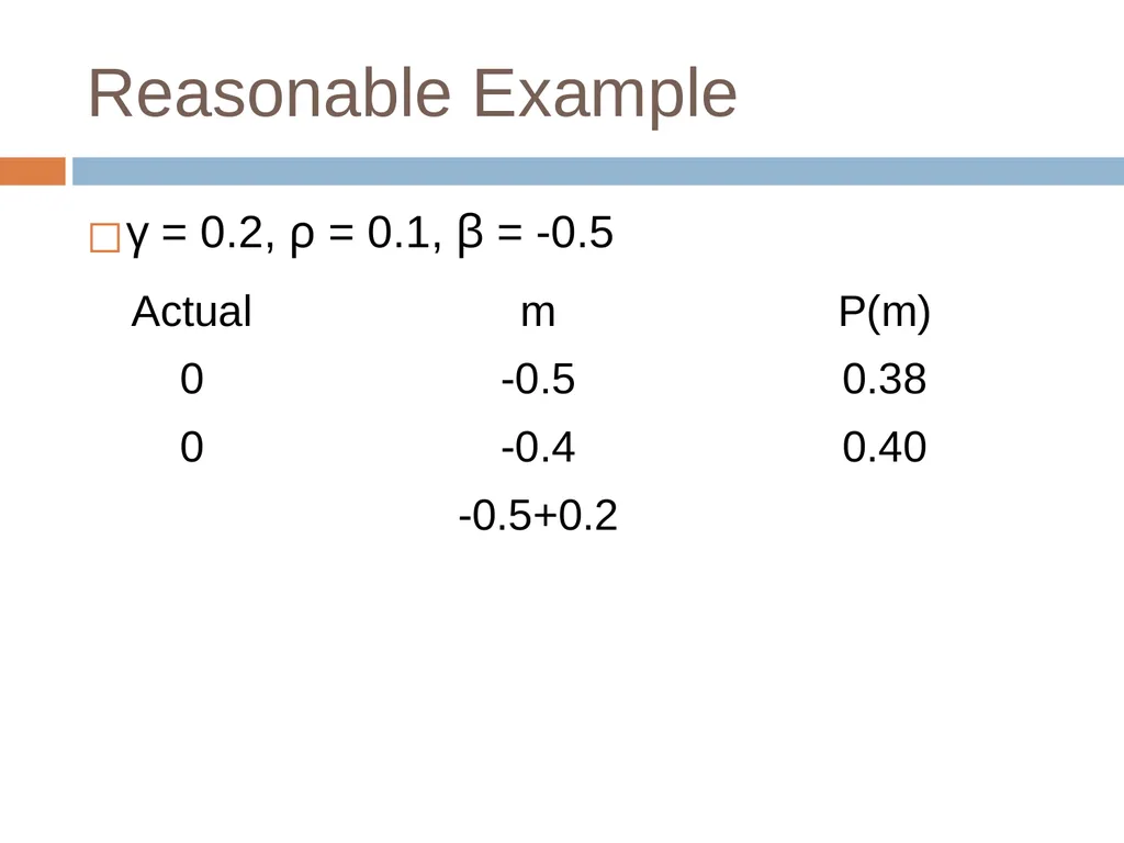
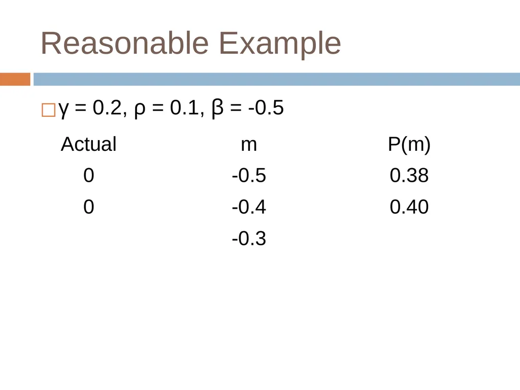
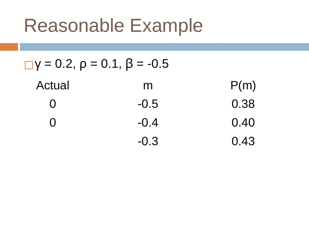
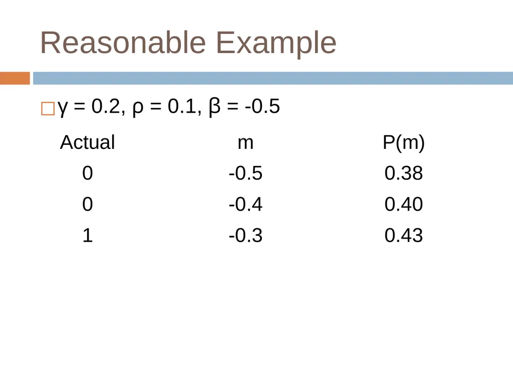
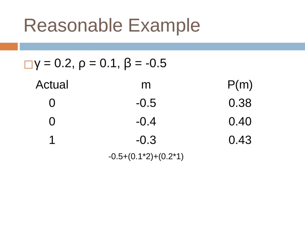
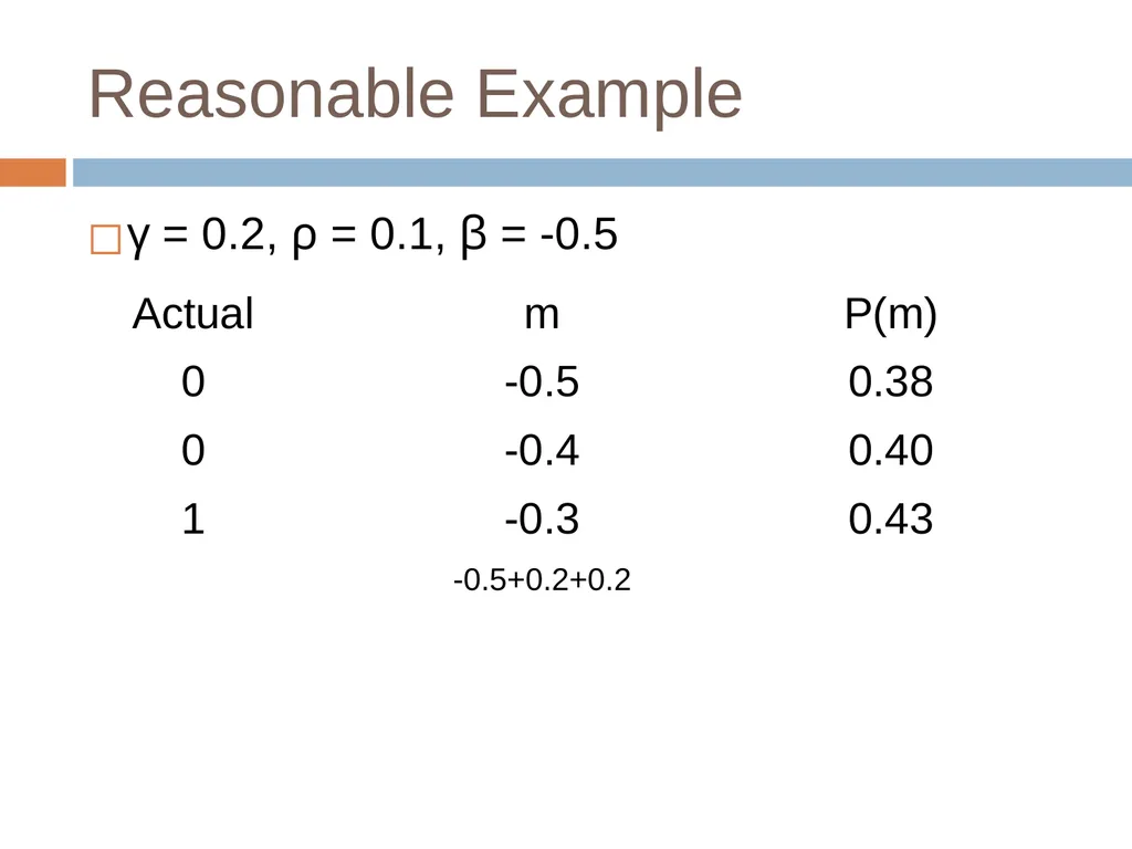
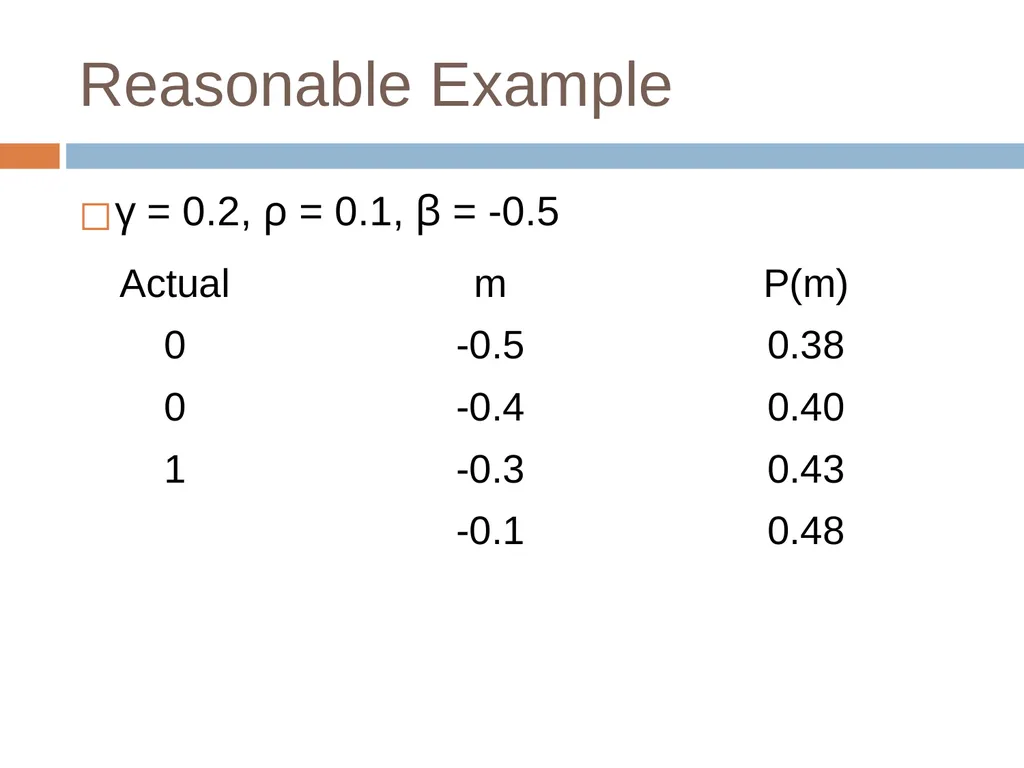
slide65. Reasonable Example γ = 0.2, ρ = 0.1, β = -0.5<br>
slide66. Reasonable Example γ = 0.2, ρ = 0.1, β = -0.5<br>
slide67. Reasonable Example γ = 0.2, ρ = 0.1, β = -0.5<br>
slide68. Reasonable Example γ = 0.2, ρ = 0.1, β = -0.5<br>
slide69. Reasonable Example γ = 0.2, ρ = 0.1, β = -0.5<br>
slide70. Reasonable Example γ = 0.2, ρ = 0.1, β = -0.5<br>
slide71. Reasonable Example γ = 0.2, ρ = 0.1, β = -0.5<br>
slide72. Reasonable Example γ = 0.2, ρ = 0.1, β = -0.5<br>
slide73. Reasonable Example γ = 0.2, ρ = 0.1, β = -0.5<br>
slide74. Reasonable Example γ = 0.2, ρ = 0.1, β = -0.5<br>
slide75. Reasonable Example γ = 0.2, ρ = 0.1, β = -0.5<br>
slide76. Reasonable Example γ = 0.2, ρ = 0.1, β = -0.5<br>
slide77. Reasonable Example γ = 0.2, ρ = 0.1, β = -0.5<br>
slide78. Reasonable Example γ = 0.2, ρ = 0.1, β = -0.5<br>
slide79. Degeneracy in PFA (Maier et al., 2021) Three degenerate cases
γ < 0
γ < ρ
γ = ρ = 0<br>
slide80. Degeneracy in PFA (Maier et al., 2021) Three degenerate cases
γ < 0
γ < ρ
γ = ρ = 0

One seemingly degenerate (but not) case
4. ρ > 0
“It is worth noting that a fourth case when ρ > 0 -- is not degenerate, due to the multiple functions the parameters perform in PFA. In this case, the rate of learning the skill may outweigh the evidence of lack of student knowledge that an incorrect answer provides. So long as γ > ρ, a positive ρ is conceptually acceptable.”<br>
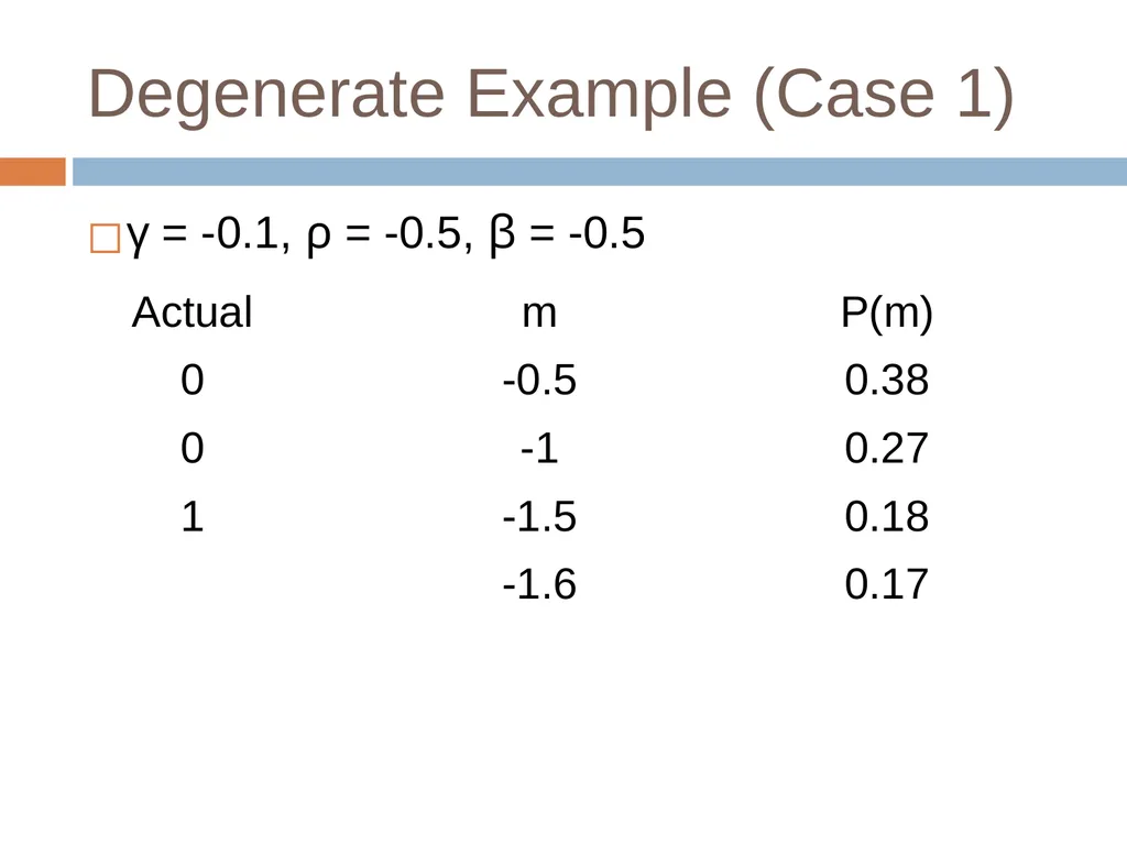
slide81. Degenerate Example (Case 1) γ = -0.1, ρ = -0.5, β = -0.5<br>
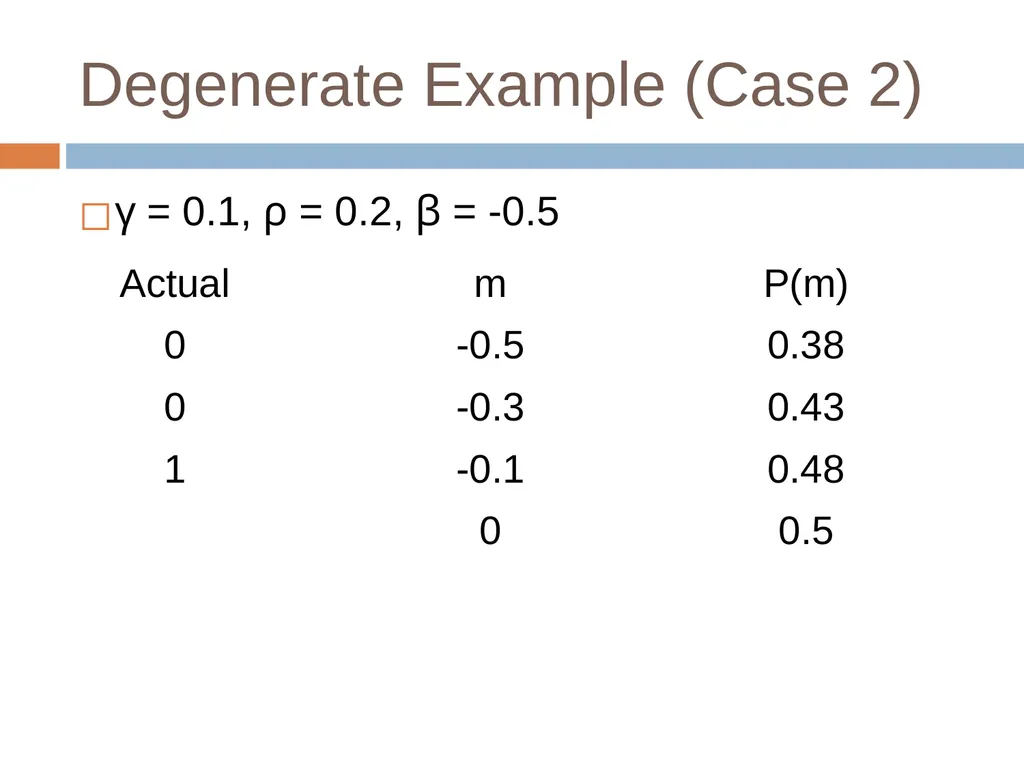
slide82. Degenerate Example (Case 2) γ = 0.1, ρ = 0.2, β = -0.5<br>
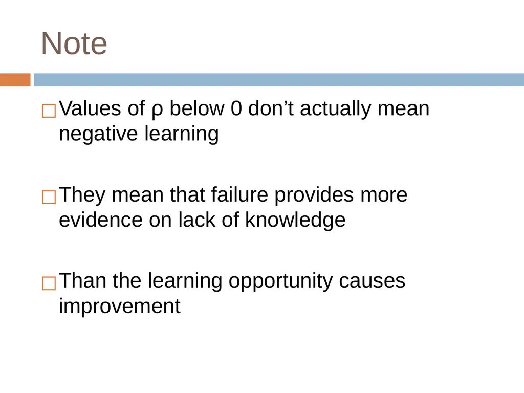
slide83. Note Values of ρ below 0 don’t actually mean negative learning

They mean that failure provides more evidence on lack of knowledge

Than the learning opportunity causes improvement<br>
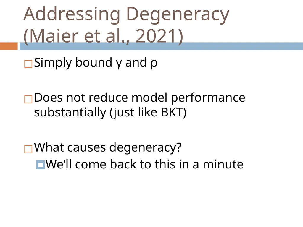
slide84. Addressing Degeneracy(Maier et al., 2021) Simply bound γ and ρ

Does not reduce model performance substantially (just like BKT)

What causes degeneracy?
We’ll come back to this in a minute<br>
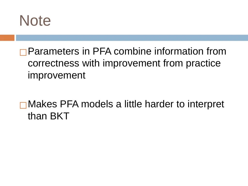
slide85. Note Parameters in PFA combine information from correctness with improvement from practice improvement

Makes PFA models a little harder to interpret than BKT<br>
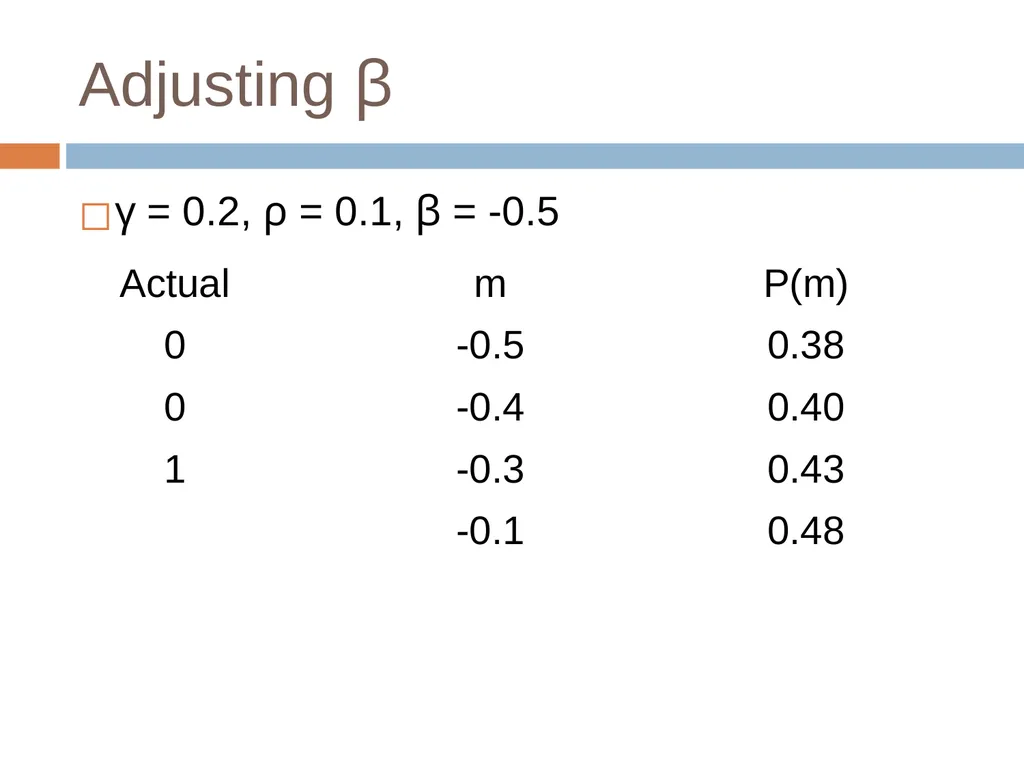
slide86. Adjusting β γ = 0.2, ρ = 0.1, β = -0.5<br>
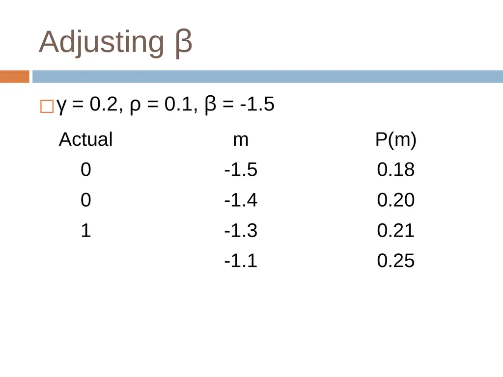
slide87. Adjusting β γ = 0.2, ρ = 0.1, β = -1.5<br>
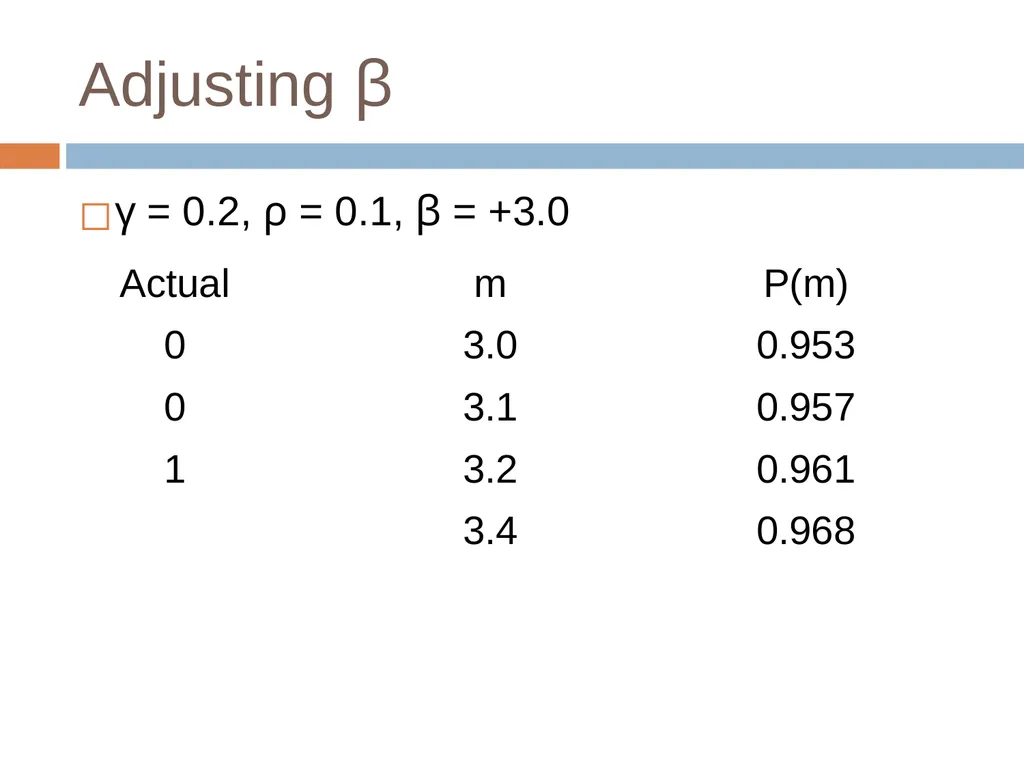
slide88. Adjusting β γ = 0.2, ρ = 0.1, β = +3.0<br>
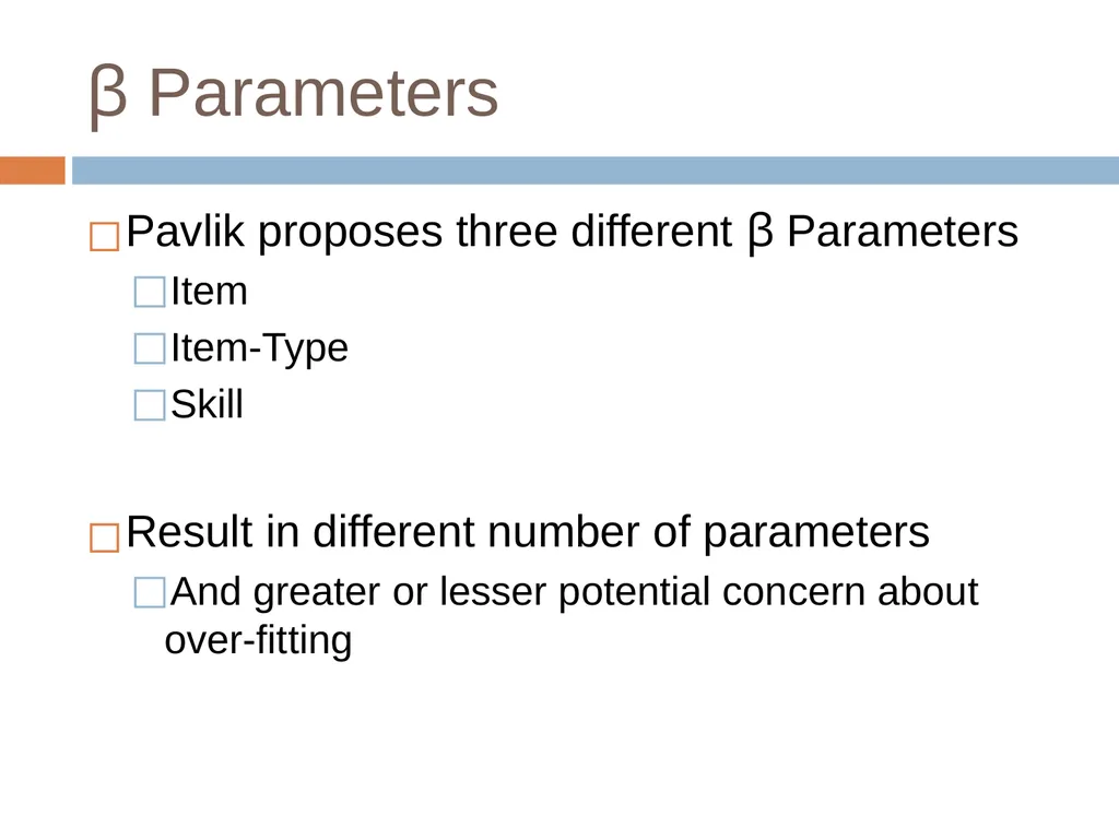
slide89. β Parameters Pavlik proposes three different β Parameters
Item
Item-Type
Skill

Result in different number of parameters
And greater or lesser potential concern about over-fitting<br>
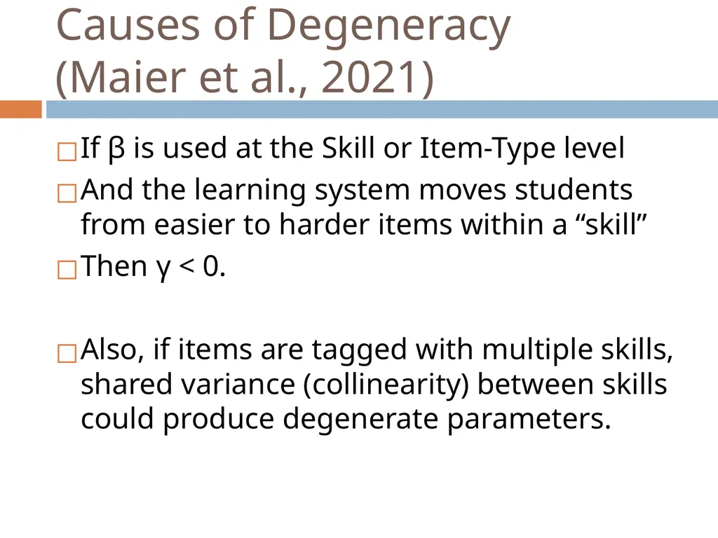
slide90. Causes of Degeneracy (Maier et al., 2021) If β is used at the Skill or Item-Type level
And the learning system moves students from easier to harder items within a “skill”
Then γ < 0.

Also, if items are tagged with multiple skills, shared variance (collinearity) between skills could produce degenerate parameters.<br>
slide91. Fitting PFA Typically Expectation Maximization is used<br>
slide92. Expectation Maximization Starts with initial values for each parameter
Estimates student correctness at each problem step
Estimates params using student correctness estimates
If goodness is substantially better than last time it was estimated, and max iterations has not been reached, go to step 2<br>
slide93. Expectation Maximization EM is vulnerable to local minima

Randomized restart typically used<br>
slide94. Is PFA better than BKT? Approximately equal predictive power across a lot of studies (Pavlik et al., 2009; Gong et al., 2010; Baker et al., 2011; Pardos et al., 2011, 2012)

Different virtues and flaws – choose the one that better fits your goals<br>
slide95. Is PFA used in the real world? Yes, but by far fewer learning systems than BKT

Maier et al. (2021) discuss its use in Reveal Math 1<br>
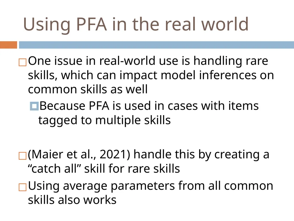
slide96. Using PFA in the real world One issue in real-world use is handling rare skills, which can impact model inferences on common skills as well
Because PFA is used in cases with items tagged to multiple skills

(Maier et al., 2021) handle this by creating a “catch all” skill for rare skills
Using average parameters from all common skills also works<br>
slide97. Final Thoughts on PFA PFA is a competitor for measuring student skill, which predicts the probability of correctness rather than latent knowledge

Can handle multiple KCs for the same item, a big virtue<br>
slide98. Beyond PFA<br>
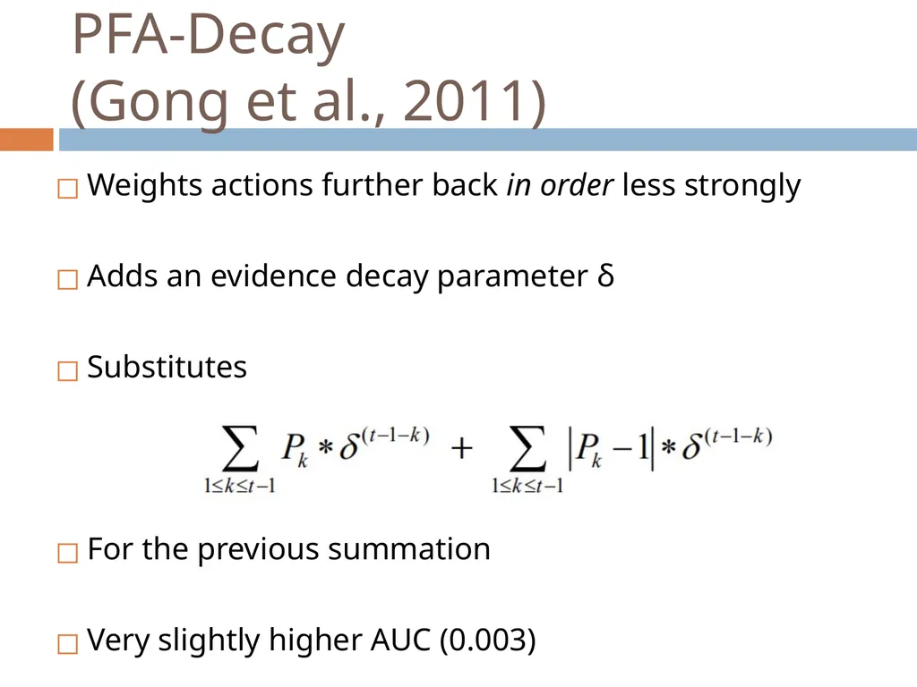
slide99. PFA-Decay (Gong et al., 2011) Weights actions further back in order less strongly

Adds an evidence decay parameter δ

Substitutes

For the previous summation

Very slightly higher AUC (0.003)<br>
slide100. R-PFA (Galyardt & Goldin, 2014) Weights actions further back in order less strongly

Looks at proportion of success-failure, weighting by distance in order from current action
Adds an evidence decay parameter b
Adds “ghost practices” before current practice to make math work

Substitutes

For the previous summation

A little higher AUC (0.003-0.027) (Pavlik et al., 2021)<br>
slide101. LKT (Pavlik et al., 2021) Creates a general framework for variants of PFA<br>
slide103. LKT (Pavlik et al., 2021) New/ongoing work on variants to PFA typically frames itself in terms of LKT components (and proposes additional components)<br>
slide104. Item Response Theory A classic approach for assessment, used for decades in tests and some online learning environments

In its classical form, has some key limitations that make it less useful for assessment in online learning
But variants such as ELO and T-IRT address some of those limitations<br>
slide105. Key goal of IRT Measuring how much of some latent trait a person has

How intelligent is Bob?
How much does Bob know about snorkeling?
SnorkelTutor<br>
slide106. Typical use of IRT Assess a student’s current knowledge of topic X

Based on a sequence of items that are dichotomously scored
E.g. the student can get a score of 0 or 1 on each item<br>
slide107. Key assumptions There is only one latent trait or skill being measured per set of items
This assumption is relaxed in the extension Cognitive Diagnosis Models (CDM)(Henson, Templin, & Willse, 2009)

No learning is occurring in between items
E.g. a testing situation with no help or feedback<br>
slide108. Key assumptions Each learner has ability θ

Each item has difficulty b and discriminability a

From these parameters, we can compute the probability P(θ) that the learner will get the item correct<br>
slide109. Note The assumption that all items tap the same latent construct, but have different difficulties

Is a very different assumption than is seen in PFA or BKT<br>
slide110. The Rasch (1PL) model Simplest IRT model, very popular

Mathematically the same model (with a different coefficient), but some different practices surrounding the math (that are out of scope for this course)

There is an entire special interest group of AERA devoted solely to the Rasch model and modeling related to Rasch (Rasch Measurement)<br>
slide111. The Rasch (1PL) model No discriminability parameter

Parameters for student ability and item difficulty<br>
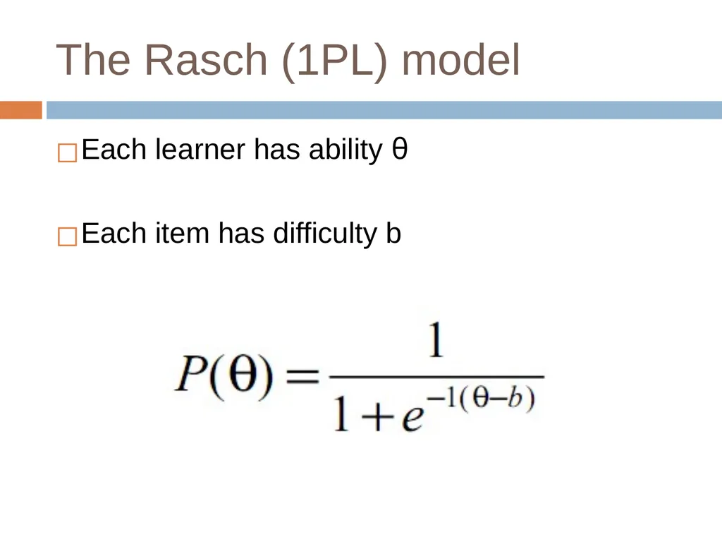
slide112. The Rasch (1PL) model Each learner has ability θ

Each item has difficulty b<br>
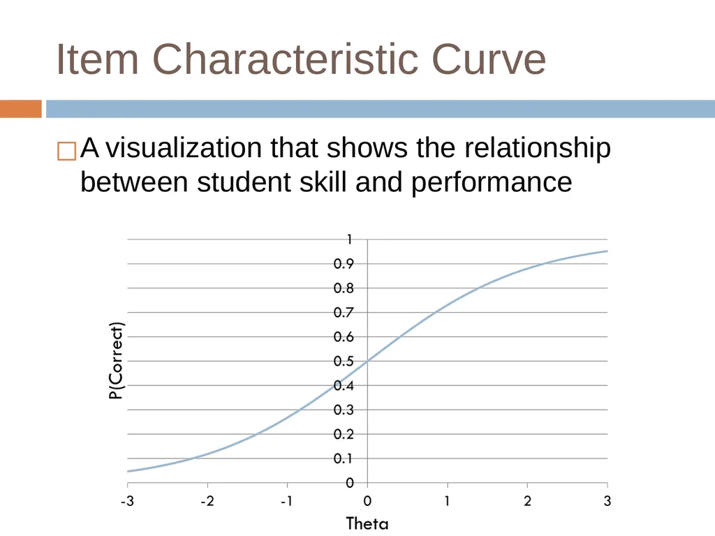
slide113. Item Characteristic Curve A visualization that shows the relationship between student skill and performance<br>
slide114. As student skill goes up, correctness goes up This graph represents b=0
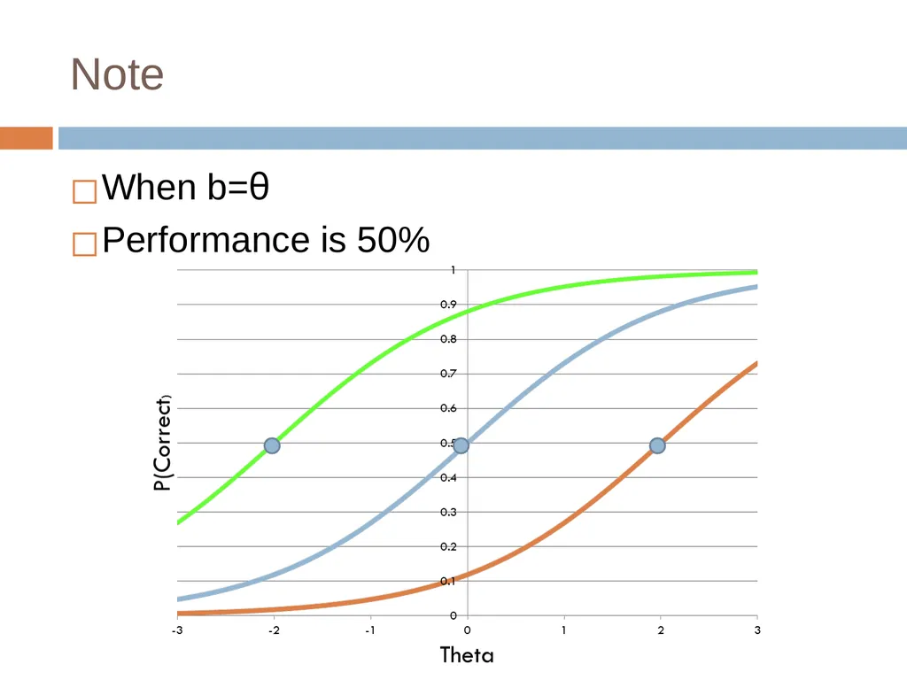
When θ=b (knowledge=difficulty), performance = 50%<br>
slide115. As student skill goes up, correctness goes up<br>
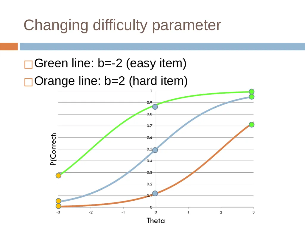
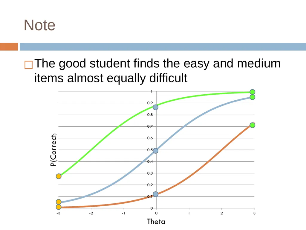
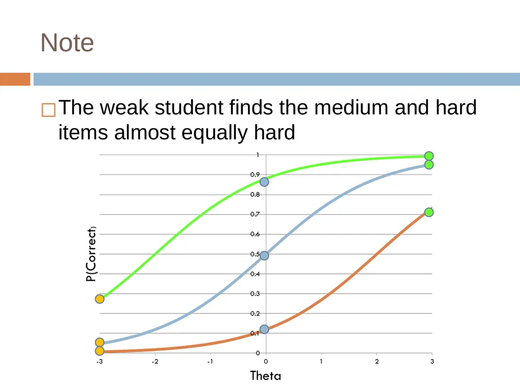
slide116. Changing difficulty parameter Green line: b=-2 (easy item)
Orange line: b=2 (hard item)<br>
slide117. Note The good student finds the easy and medium items almost equally difficult<br>
slide118. Note The weak student finds the medium and hard items almost equally hard<br>
slide119. Note When b=θ
Performance is 50%<br>
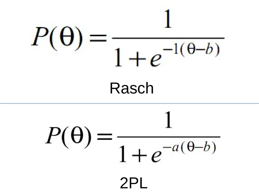
slide120. The 2PL model Another simple IRT model, very popular

Discriminability parameter a added<br>
slide121. Rasch 2PL<br>
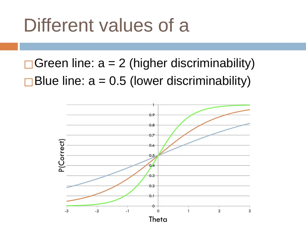
slide122. Different values of a Green line: a = 2 (higher discriminability)
Blue line: a = 0.5 (lower discriminability)<br>
slide123. Extremely high and low discriminability a=0
a approaches infinity<br>
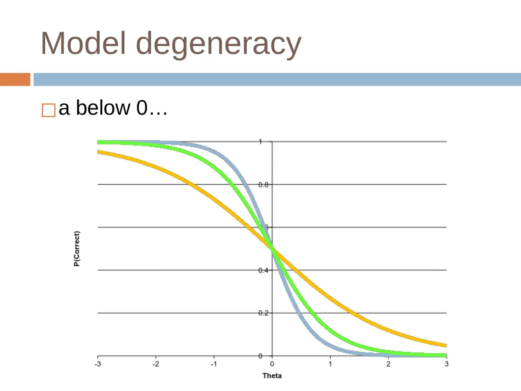
slide124. Model degeneracy a below 0…<br>
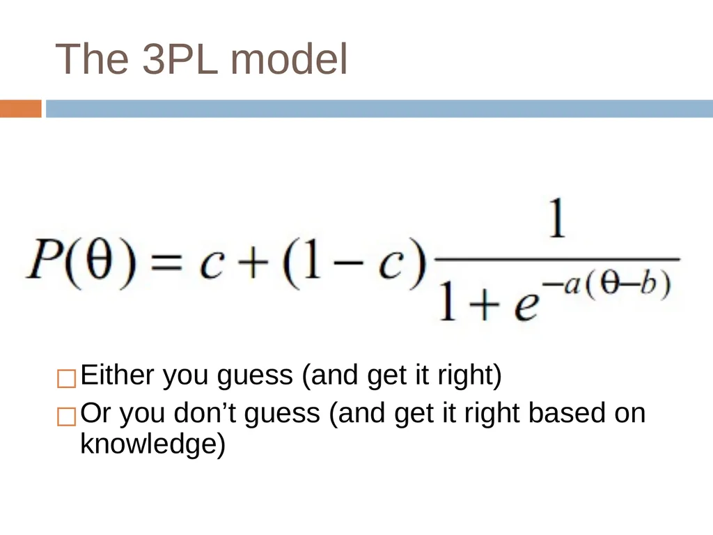
slide125. The 3PL model A more complex model

Adds a guessing parameter c<br>
slide126. The 3PL model Either you guess (and get it right)
Or you don’t guess (and get it right based on knowledge)<br>
slide127. Fitting an IRT model Can be done with Expectation Maximization
As discussed in previous lectures

Estimate knowledge and difficulty together
Then, given item difficulty estimates, you can assess a student’s knowledge in real time<br>
slide128. Uses… IRT is used quite a bit in computer-adaptive testing

Not used quite so often in online learning, where student knowledge is changing as we assess it
For those situations, BKT and PFA are more popular<br>
slide129. ELO (Elo, 1978; Pelanek, 2016) A variant of the Rasch model which can be used in a running system

Continually estimates item difficulty and student ability, updating both every time a student encounters an item<br>
slide130. ELO (Elo, 1978; Pelanek, 2016)<br>
slide131. Multivariate ELO (Abdi et al., 2019) Allows an item to involve multiple skills

Averages difficulty across skills<br>
slide132. MV-Glicko (Abdi et al., 2021) Allows an item to involve multiple skills

Averages difficulty across skills

Takes time between practices of a skill into account (much like LKT extensions to PFA)<br>
slide133. Deep Knowledge Tracing (DKT)(Piech et al., 2015) Based on long short term memory networks

Fits on sequence of student performance across skills
Predicts performance on future items within system

Can fit very complex functions
Very complex relationships between items over time<br>
slide134. DKT Initial paper reported massively better performance than original BKT or PFA (Piech et al., 2015)

Seemed at first too good to be true, and (Xiong et al., 2016) reported that (Piech et al., 2015) had used the same data points for both training and test<br>
slide135. DKT (Khajah et al., 2016) compared DKT to modern extensions to BKT on same data set
Particularly beneficial to re-fit item-skill mappings

(Wilson et al., 2016) compared DKT to temporal IRT on same data set

Bottom line: All three approaches appeared to perform comparably well<br>
slide136. But this was the beginning of what could be called DKT-Family algorithms A range of knowledge tracing algorithms based on different variants on Deep Learning

Now literally hundreds of published variants
Most of them tiny tweaks to get tiny gains in performance
But in aggregate, there appear to be some real improvements to predictive performance (see comparison in Gervet et al., 2020 for example)

I will discuss some of the key issues that researchers have tried to address, and what their approaches were<br>
slide137. Degenerate behavior (Yeung & Yeung, 2018) reported degenerate behavior for DKT
Getting answers right leads to lower knowledge
Wild swings in probability estimates in short periods of time<br>
slide138. Degenerate behavior (Yeung & Yeung, 2018) reported degenerate behavior for DKT
Getting answers right leads to lower knowledge
Wild swings in probability estimates in short periods of time

They proposed adding two types of regularization to moderate these swings
Increasing weight of current prediction for future prediction
Reducing amount model is allowed to change future estimates<br>
slide139. Impossible to interpret in terms of skills DKT Family predicts individual item correctness, not skills

What do you do for entirely new items?

What information can you provide teachers?<br>
slide140. Extension for Latent Knowledge Estimation (Zhang et al., 2017) proposed an extension to DKT, called DKVMN, that fits an item-skill mapping too
Based on Memory-Augmented Neural Network, that keeps an external memory matrix that neurons update and refer back to
Latent skill difficult to interpret<br>
slide141. Extension for Latent Knowledge Estimation (Lee & Yeung, 2019) proposed an alternative to DKT, called KQN, that attempts to output more interpretable latent skill estimates
Again, fits an external memory network to fit skills
Also attempts to fit amount of information transfer between skills

Still not that interpretable<br>
slide142. Extension for Latent Knowledge Estimation (Scruggs et al., 2020) proposed an extension to any DKT-family algorithm
Human-derived skill-item mapping used
Predicted performance on all items in skill averaged
Including both unseen and already-seen items

Led to successful prediction of post-tests outside the learning system<br>
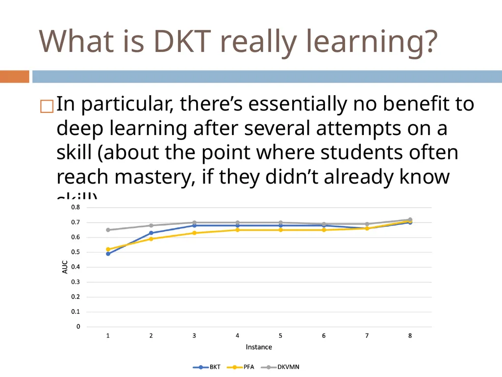
slide143. What is DKT really learning? Ding & Larson (2019) demonstrated theoretically that a lot of what DKT learns is how good a student is overall<br>
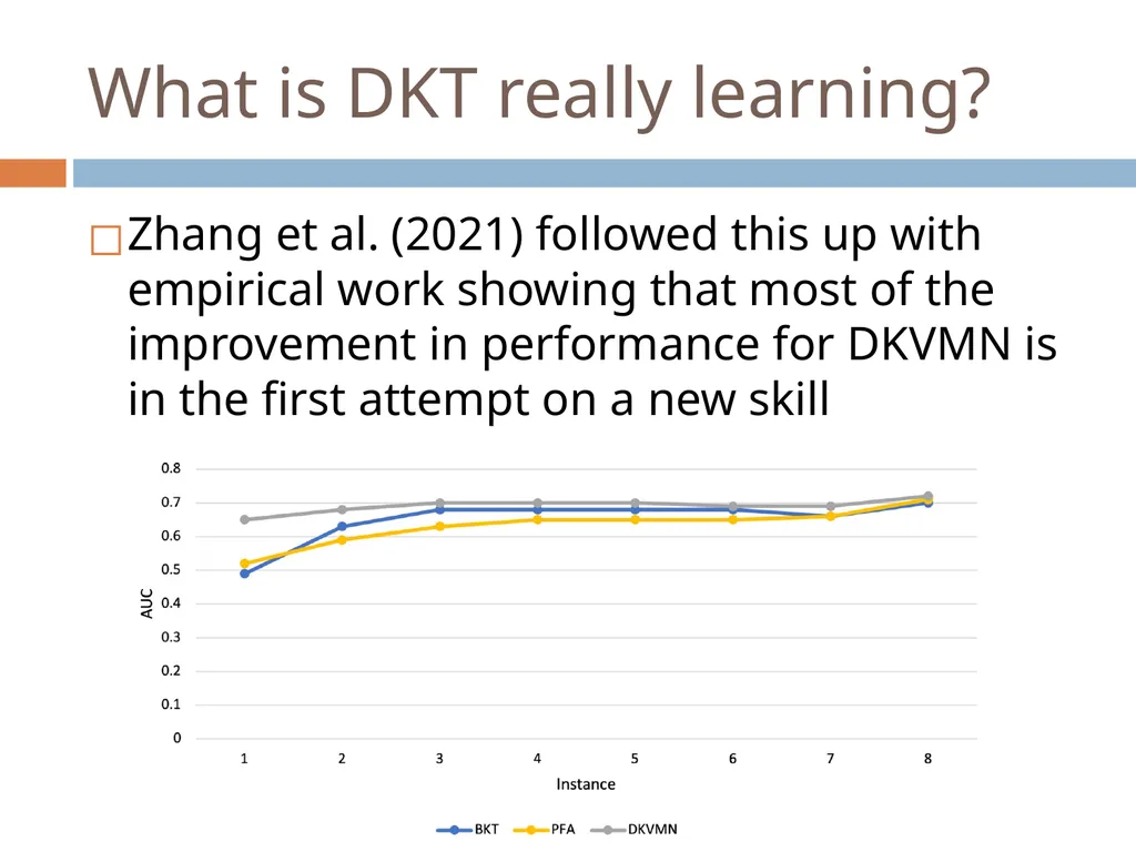
slide144. What is DKT really learning? Zhang et al. (2021) followed this up with empirical work showing that most of the improvement in performance for DKVMN is in the first attempt on a new skill<br>
slide145. What is DKT really learning? In particular, there’s essentially no benefit to deep learning after several attempts on a skill (about the point where students often reach mastery, if they didn’t already know skill)<br>
slide146. Other Important DKT variants: SAKT Pandey & Karypis (2019) proposed a DKT variant, called SAKT, which fits attentional weights between exercises and more explicitly predicts performance on current exercise from performance on past exercises
Gets a little better fit, doubles down a little more on some limitations we’ve already discussed<br>
slide147. Other Important DKT variants: AKT Ghosh et al. (2020) proposed a DKT variant, called AKT, which
Explicitly stores and uses learner’s entire past practice history for each prediction
Uses exponential decay curve to downweight past actions
Uses Rasch-model embeddings to calculate item difficulty<br>
slide148. Adding in more information: SAINT+ Shin et al. (2021) added elapsed time and lag time as additional inputs, leading to better performance<br>
slide149. Adding in more information: Process-BERT Scarlatos et al. (2022) added timing and use of resources such as calculator

Additional information leads to better performance<br>
slide150. Curious methodological note Most DKT-family papers report large improvements over previous algorithms, including other DKT-family algorithms

Improvements that seem to mostly or entirely dissipate in the next paper<br>
slide151. Some reasons Poor validation and over-fitting

A lot of DKT-family papers don’t use student-level cross-validation
Poor cross-validation benefits DKT-family algorithms more than other algorithms, because DKT-family fits more aggressively

A lot of DKT-family papers fit their own hyperparameters but use past hyperparameters for other algorithms<br>
slide152. An evaluation Gervet et al. (2020) compares KT algorithms on several data sets
Key findings
Different data sets have different winners
DKT-family performs better than other algorithms on large data sets, but worse on smaller data sets
DKT-family algorithms perform worse than LKT-family on data sets with very high numbers of practices per skill (i.e. language learning)
DKT-family algorithms do better at predicting if exact order of items matters (which can occur if items within a skill vary a lot)
DKT-family algorithms reach peak performance faster than other algorithms (also seen in Zhang et al., 2021)<br>
slide153. Next Frontier for DKT-family: Beyond Correctness Option Tracing (Ghosh et al., 2021) extends output layer to predict which multiple choice item the student will select<br>
slide154. Next Frontier for DKT-family: Beyond Correctness Open-Ended Knowledge Tracing (Liu et al., 2022) integrates KT with
A GPT-2 model fine-tuned on 2.1 million Java code exercises and written descriptions of them

In order to generate predicted student code which makes predicted specific errors<br>
slide155. DKT-family: work continues Dozens of recent papers trying to get better results by adjusting the deep learning framework in various ways<br>
slide156. Is future correctness enough? Up until this point we’ve been talking about predicting future correctness<br>
slide157. But what if you forget it tomorrow? Another way to look at knowledge is – how long will you remember it?<br>
slide158. Relevant for all knowledge Mostly studied in the context of memory for facts, rather than skills

How do you say banana in Spanish?
What is the capital of New York?
Where are the Islands of Langerhans?<br>
slide159. Spacing Effect It has long been known that spaced practice (i.e. pausing between studying the same fact) is better than massed practice (i.e. cramming)

Early adaptive systems implemented this behavior in simple ways (i.e. Leitner, 1972)<br>
slide160. ACT-R Memory Equations (Pavlik & Anderson, 2005) Memory duration can be understood in terms of memory strength (referred to as activation)<br>
slide161. ACT-R Memory Equations (Pavlik & Anderson, 2005)<br>
slide162. ACT-R Memory Equations (Pavlik & Anderson, 2005)<br>
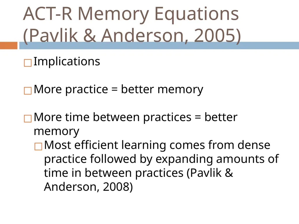
slide163. ACT-R Memory Equations (Pavlik & Anderson, 2005) Implications

More practice = better memory

More time between practices = better memory
Most efficient learning comes from dense practice followed by expanding amounts of time in between practices (Pavlik & Anderson, 2008)<br>
slide164. MCM (Mozer et al., 2009) Postulates that decay speed drops, the more times a fact is encountered

Functionally complex model where

Knowledge strength (and therefore probability of remembering) is a function of the sum of the traces’ actual contributions, divided by the product of their potential contributions

Power function is estimated as a combination of exponential functions<br>
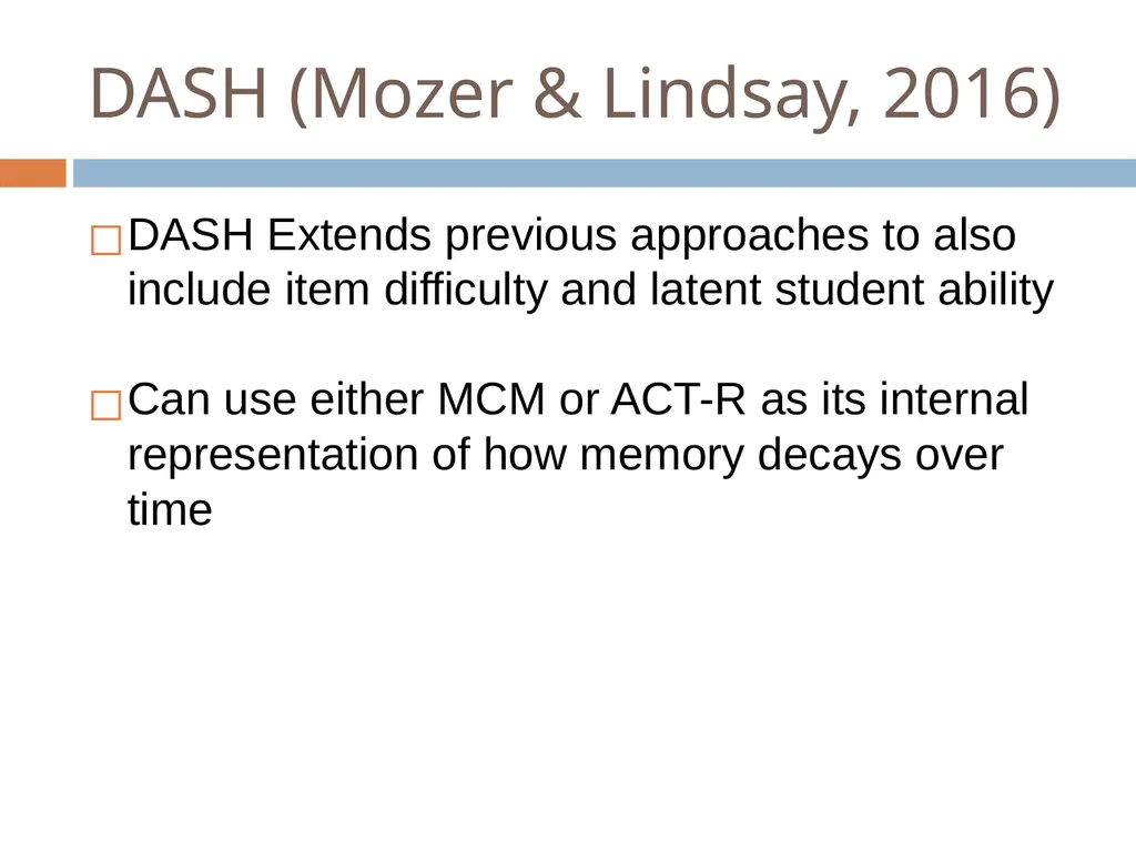
slide165. DASH (Mozer & Lindsay, 2016) DASH Extends previous approaches to also include item difficulty and latent student ability

Can use either MCM or ACT-R as its internal representation of how memory decays over time<br>
slide166. Duolingo (Settles & Mercer, 2016) Fits regression model to predict both recall and estimated half-life of memory (based on lag time)

Based on estimate of exponential decay of memory<br>
slide167. Duolingo (Settles & Mercer, 2016) Uses feature set including
Time since word last seen
Total number of times student has seen the word
Total number of times student has correctly recalled the word
Total number of times student has failed to recalled the word
Word difficulty<br>