
Lecture 15: Query Optimization 1 Announcements
TA
Published · 49 slides · 0 views
1 / 1
Description
Lecture 15: Query Optimization 1 Announcements Today, right after lecture, exam review in this room for 30 minutes. Additional questions in office hours. Scheduling: Im away next week Old Plan: Zhongrui 1 canceled class. New Plan: In
Related Topics
Download this presentation From Below
"Lecture 15: Query Optimization 1 Announcements" is the property of its rightful owner. Permission is granted to download and print the materials on this website for personal, non-commercial use only, and to display it on your personal computer provided you do not modify the materials and that you retain all copyright notices contained in the materials. By downloading content from our website, you accept the terms of this agreement.
Share
Embed code
Presentation Transcript
01
Lecture 15: Query Optimization 1<br>
02
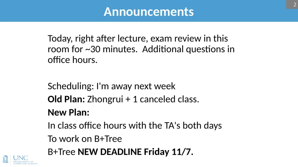
Announcements Today, right after lecture, exam review in this room for ~30 minutes. Additional questions in office hours.
Scheduling: I'm away next week
Old Plan: Zhongrui + 1 canceled class.
New Plan:
In class office hours with the TA's both days
To work on B+Tree
B+Tree NEW DEADLINE Friday 11/7. 2<br>
Scheduling: I'm away next week
Old Plan: Zhongrui + 1 canceled class.
New Plan:
In class office hours with the TA's both days
To work on B+Tree
B+Tree NEW DEADLINE Friday 11/7. 2<br>
03
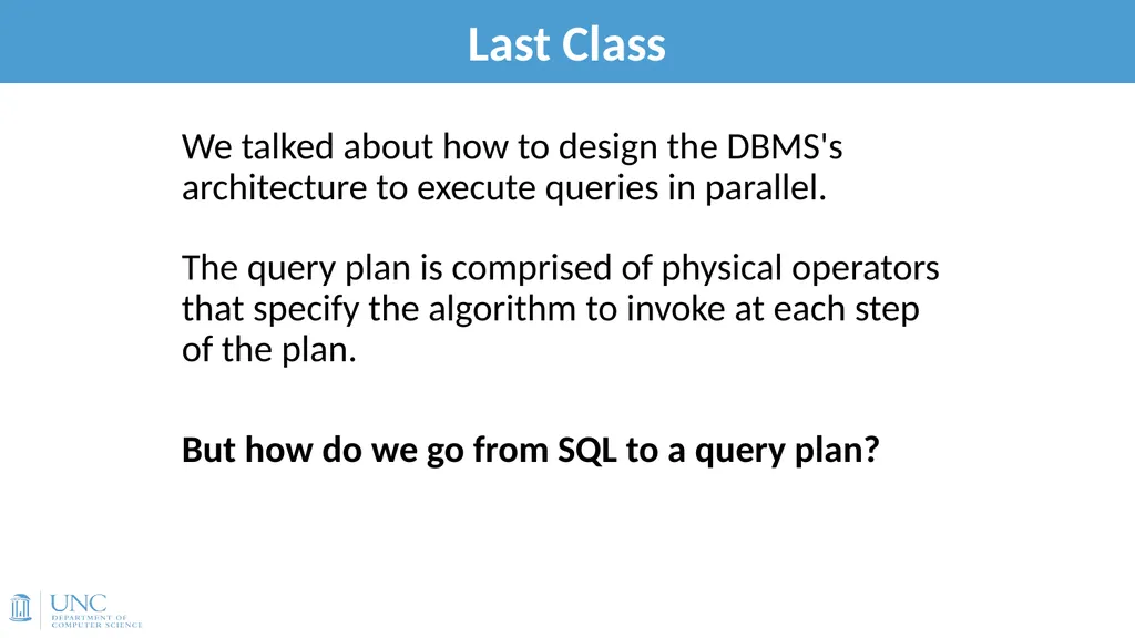
Last Class We talked about how to design the DBMS's architecture to execute queries in parallel.
The query plan is comprised of physical operators that specify the algorithm to invoke at each step of the plan.
But how do we go from SQL to a query plan? 3<br>
The query plan is comprised of physical operators that specify the algorithm to invoke at each step of the plan.
But how do we go from SQL to a query plan? 3<br>
04
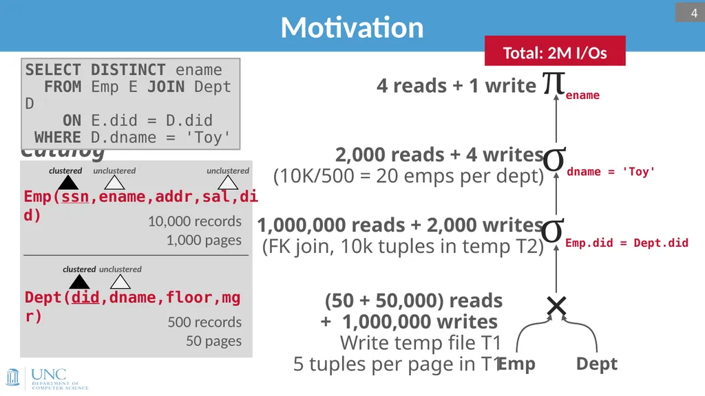
1,000,000 reads + 2,000 writes
(FK join, 10k tuples in temp T2) 2,000 reads + 4 writes
(10K/500 = 20 emps per dept) Motivation 4 4 reads + 1 write Total: 2M I/Os SELECT DISTINCT ename
FROM Emp E JOIN Dept D
ON E.did = D.did
WHERE D.dname = 'Toy' (50 + 50,000) reads + 1,000,000 writes
Write temp file T1 5 tuples per page in T1<br>
WHERE D.dname = 'Toy' (50 + 50,000) reads + 1,000,000 writes
Write temp file T1 5 tuples per page in T1<br>
05
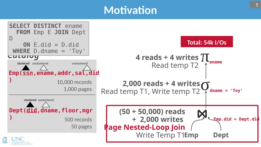
2,000 reads + 4 writes
Read temp T1, Write temp T2 4 reads + 4 writes
Read temp T2 Motivation 5 Total: 54k I/Os SELECT DISTINCT ename
FROM Emp E JOIN Dept D
ON E.did = D.did
WHERE D.dname = 'Toy' Emp Dept πename σdname = 'Toy' ⋈Emp.did = Dept.did (50 + 50,000) reads + 2,000 writes
Page Nested-Loop Join Write Temp T1 clustered unclustered unclustered<br>
WHERE D.dname = 'Toy' Emp Dept πename σdname = 'Toy' ⋈Emp.did = Dept.did (50 + 50,000) reads + 2,000 writes
Page Nested-Loop Join Write Temp T1 clustered unclustered unclustered<br>
06
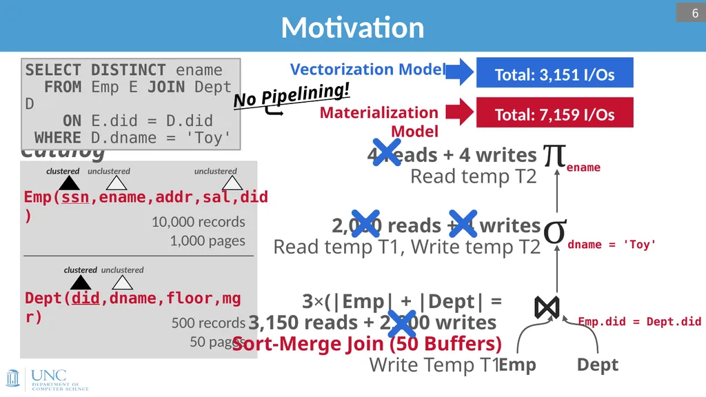
2,000 reads + 4 writes
Read temp T1, Write temp T2 4 reads + 4 writes
Read temp T2 Motivation 6 Total: 7,159 I/Os SELECT DISTINCT ename
FROM Emp E JOIN Dept D
ON E.did = D.did
WHERE D.dname = 'Toy' Emp Dept πename σdname = 'Toy' ⋈Emp.did = Dept.did 3×(|Emp| + |Dept| = 3,150 reads + 2,000 writes
Sort-Merge Join (50 Buffers) Write Temp T1 Materialization Model Total: 3,151 I/Os Vectorization Model clustered unclustered unclustered No Pipelining!<br>
WHERE D.dname = 'Toy' Emp Dept πename σdname = 'Toy' ⋈Emp.did = Dept.did 3×(|Emp| + |Dept| = 3,150 reads + 2,000 writes
Sort-Merge Join (50 Buffers) Write Temp T1 Materialization Model Total: 3,151 I/Os Vectorization Model clustered unclustered unclustered No Pipelining!<br>
07
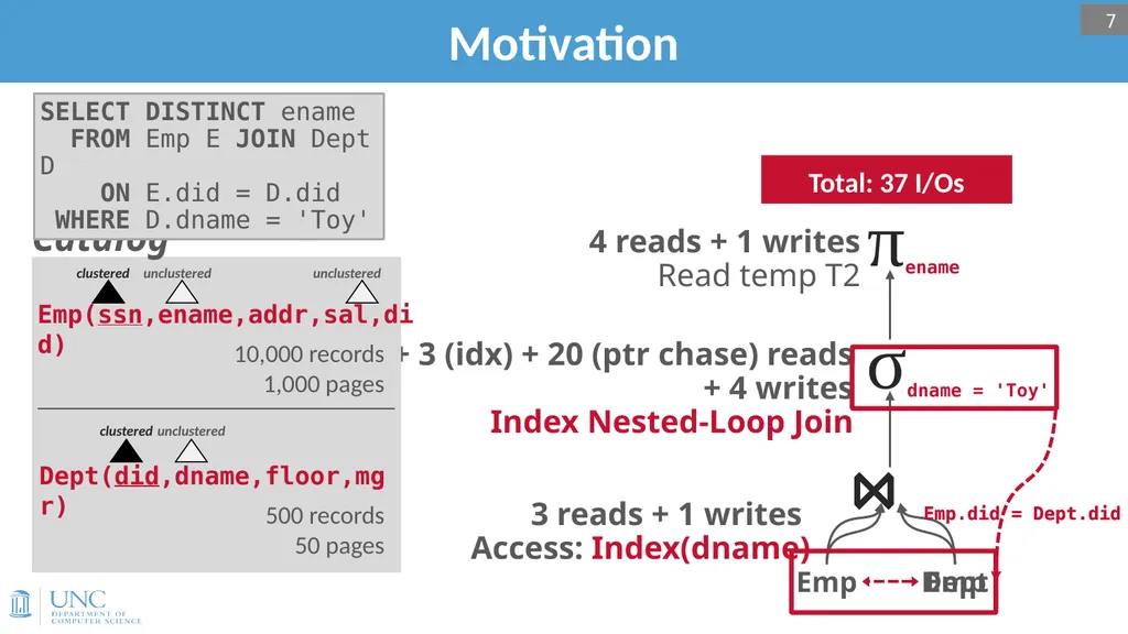
1 + 3 (idx) + 20 (ptr chase) reads
+ 4 writes
Index Nested-Loop Join 4 reads + 1 writes
Read temp T2 Motivation 7 Total: 37 I/Os SELECT DISTINCT ename
FROM Emp E JOIN Dept D
ON E.did = D.did
WHERE D.dname = 'Toy' Emp Dept πename 3 reads + 1 writes
Access: Index(dname) clustered unclustered unclustered<br>
WHERE D.dname = 'Toy' Emp Dept πename 3 reads + 1 writes
Access: Index(dname) clustered unclustered unclustered<br>
08
Today's Agenda Background
Heuristic / Ruled-based Optimization
Cost-based Optimization
Cost Model Estimation
Warning #1: This is hard.
Warning #2: There could be a whole course in this, we have one lecture. 8<br>
Heuristic / Ruled-based Optimization
Cost-based Optimization
Cost Model Estimation
Warning #1: This is hard.
Warning #2: There could be a whole course in this, we have one lecture. 8<br>
09
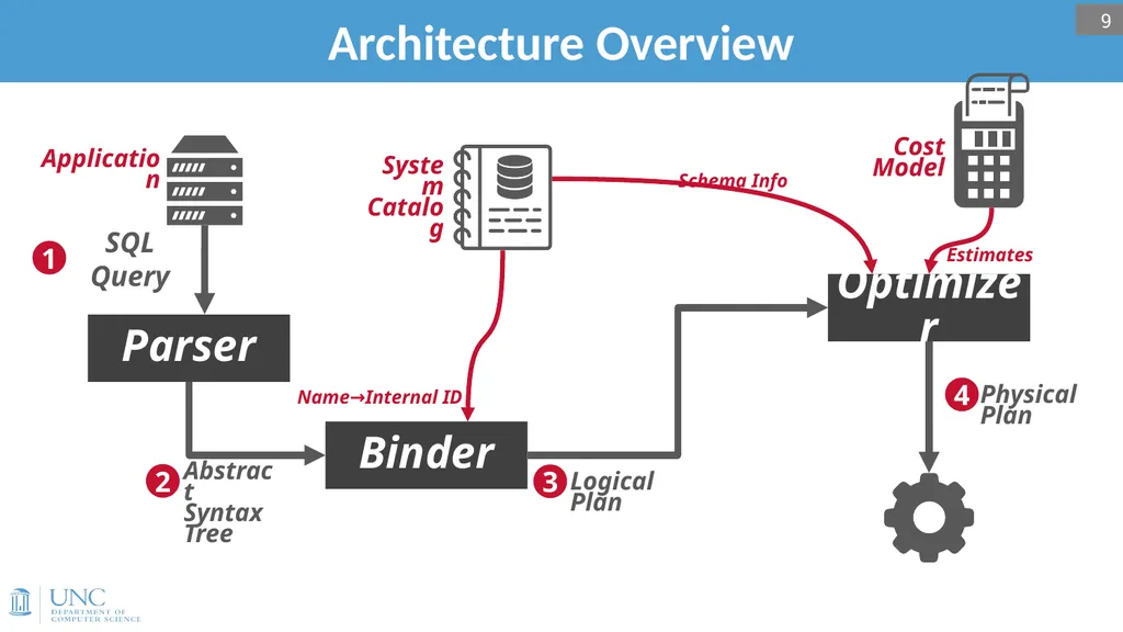
Architecture Overview 9 Parser Application Name→Internal ID Schema Info Estimates<br>
10
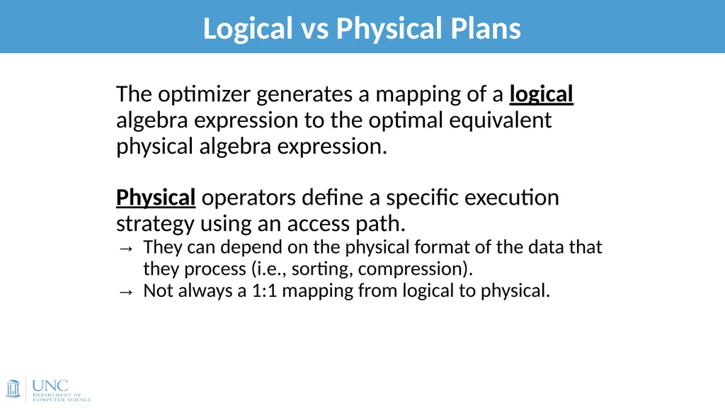
Logical vs Physical Plans The optimizer generates a mapping of a logical algebra expression to the optimal equivalent physical algebra expression.
Physical operators define a specific execution strategy using an access path.
They can depend on the physical format of the data that they process (i.e., sorting, compression).
Not always a 1:1 mapping from logical to physical. 10<br>
Physical operators define a specific execution strategy using an access path.
They can depend on the physical format of the data that they process (i.e., sorting, compression).
Not always a 1:1 mapping from logical to physical. 10<br>
11
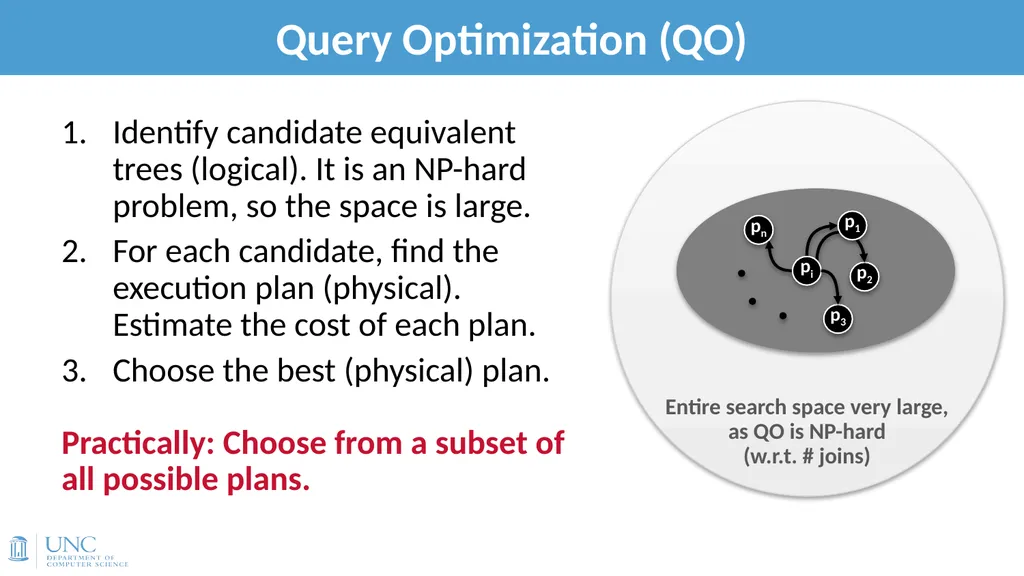
Query Optimization (QO) Identify candidate equivalent trees (logical). It is an NP-hard problem, so the space is large.
For each candidate, find the execution plan (physical). Estimate the cost of each plan.
Choose the best (physical) plan.
Practically: Choose from a subset of all possible plans. 11 CS 564: Database Management Systems; (c) Jignesh M. Patel, 2013<br>
For each candidate, find the execution plan (physical). Estimate the cost of each plan.
Choose the best (physical) plan.
Practically: Choose from a subset of all possible plans. 11 CS 564: Database Management Systems; (c) Jignesh M. Patel, 2013<br>
12
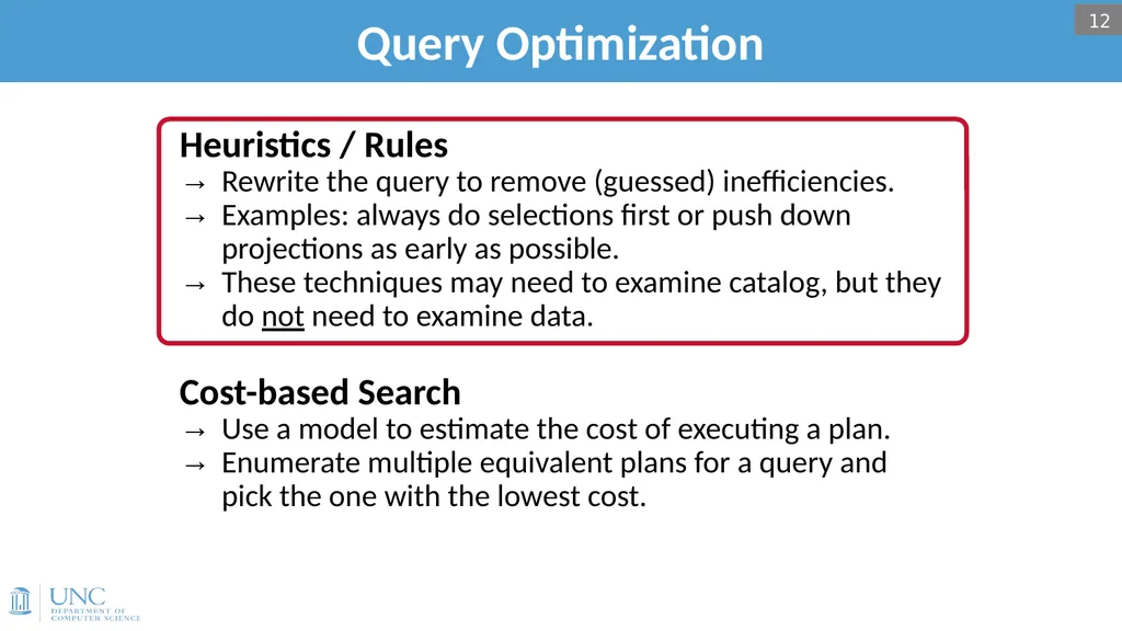
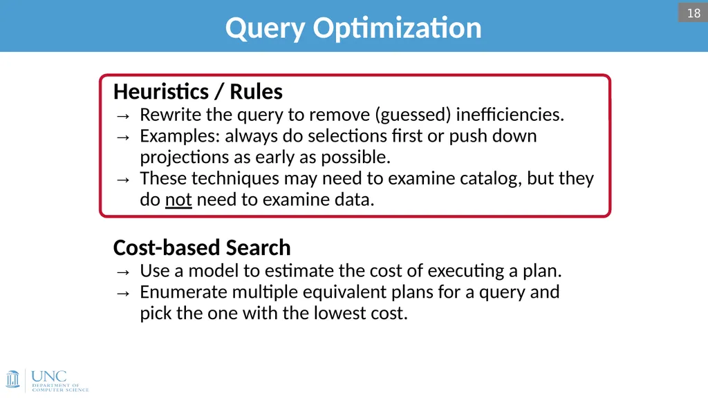
Query Optimization Heuristics / Rules
Rewrite the query to remove (guessed) inefficiencies.
Examples: always do selections first or push down projections as early as possible.
These techniques may need to examine catalog, but they do not need to examine data.
Cost-based Search
Use a model to estimate the cost of executing a plan.
Enumerate multiple equivalent plans for a query and pick the one with the lowest cost. 12<br>
Rewrite the query to remove (guessed) inefficiencies.
Examples: always do selections first or push down projections as early as possible.
These techniques may need to examine catalog, but they do not need to examine data.
Cost-based Search
Use a model to estimate the cost of executing a plan.
Enumerate multiple equivalent plans for a query and pick the one with the lowest cost. 12<br>
13
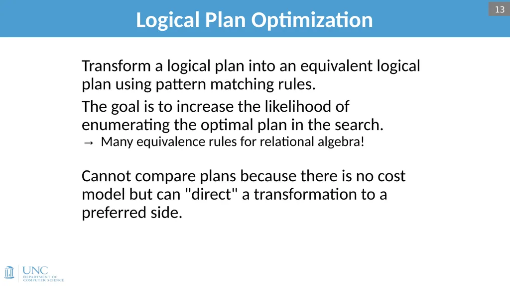
Logical Plan Optimization Transform a logical plan into an equivalent logical plan using pattern matching rules.
The goal is to increase the likelihood of enumerating the optimal plan in the search.
Many equivalence rules for relational algebra!
Cannot compare plans because there is no cost model but can "direct" a transformation to a preferred side. 13<br>
The goal is to increase the likelihood of enumerating the optimal plan in the search.
Many equivalence rules for relational algebra!
Cannot compare plans because there is no cost model but can "direct" a transformation to a preferred side. 13<br>
14
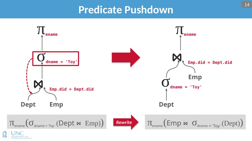
Predicate Pushdown 14 πename (σdname = 'Toy' (Dept ⋈ Emp)) πename (Emp ⋈ σdname = 'Toy' (Dept)) Rewrite<br>
15
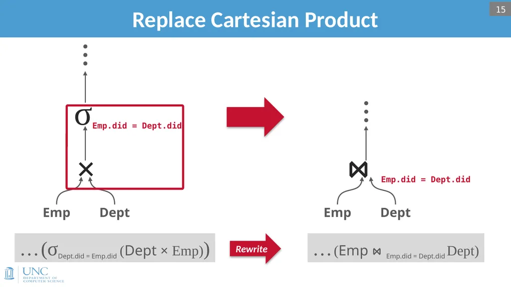
Replace Cartesian Product 15 … (σDept.did = Emp.did (Dept × Emp)) Rewrite<br>
16
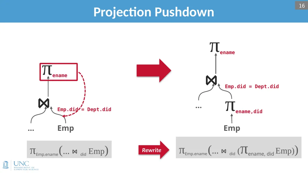
Projection Pushdown 16 πEmp.ename (… ⋈did Emp) Rewrite<br>
17
Equivalence P1 (P2(R)) ≡ P2 (P1(R)) ( commutativity)
P1⋀P2 … ⋀Pn (R) ≡ P1(P2( … Pn(R))) (cascading )
∏a1(R) ≡ ∏a1(∏a2(…∏ak (R)…)), ai ⊆ ai+1 (cascading ∏)
R ⋈ S ≡ S ⋈ R (join commutativity)
R ⋈ (S ⋈ T) ≡ (R ⋈ S) ⋈ T (join associativity)
P (R X S) ≡ (R ⋈P S), if P is a join predicate
P (R X S) ≡ P1 (P2(R) ⋈P4 P3(S)) , where P = p1 ∧ p2 ∧ p3 ∧ p4
∏A1,A2,…An(P (R)) ≡ ∏A1,A2,…An(P (∏A1,…An, B1,… BMR)), where B1 … BM are columns in P
… 17<br>
P1⋀P2 … ⋀Pn (R) ≡ P1(P2( … Pn(R))) (cascading )
∏a1(R) ≡ ∏a1(∏a2(…∏ak (R)…)), ai ⊆ ai+1 (cascading ∏)
R ⋈ S ≡ S ⋈ R (join commutativity)
R ⋈ (S ⋈ T) ≡ (R ⋈ S) ⋈ T (join associativity)
P (R X S) ≡ (R ⋈P S), if P is a join predicate
P (R X S) ≡ P1 (P2(R) ⋈P4 P3(S)) , where P = p1 ∧ p2 ∧ p3 ∧ p4
∏A1,A2,…An(P (R)) ≡ ∏A1,A2,…An(P (∏A1,…An, B1,… BMR)), where B1 … BM are columns in P
… 17<br>
18
Query Optimization Heuristics / Rules
Rewrite the query to remove (guessed) inefficiencies.
Examples: always do selections first or push down projections as early as possible.
These techniques may need to examine catalog, but they do not need to examine data.
Cost-based Search
Use a model to estimate the cost of executing a plan.
Enumerate multiple equivalent plans for a query and pick the one with the lowest cost. 18<br>
Rewrite the query to remove (guessed) inefficiencies.
Examples: always do selections first or push down projections as early as possible.
These techniques may need to examine catalog, but they do not need to examine data.
Cost-based Search
Use a model to estimate the cost of executing a plan.
Enumerate multiple equivalent plans for a query and pick the one with the lowest cost. 18<br>
19
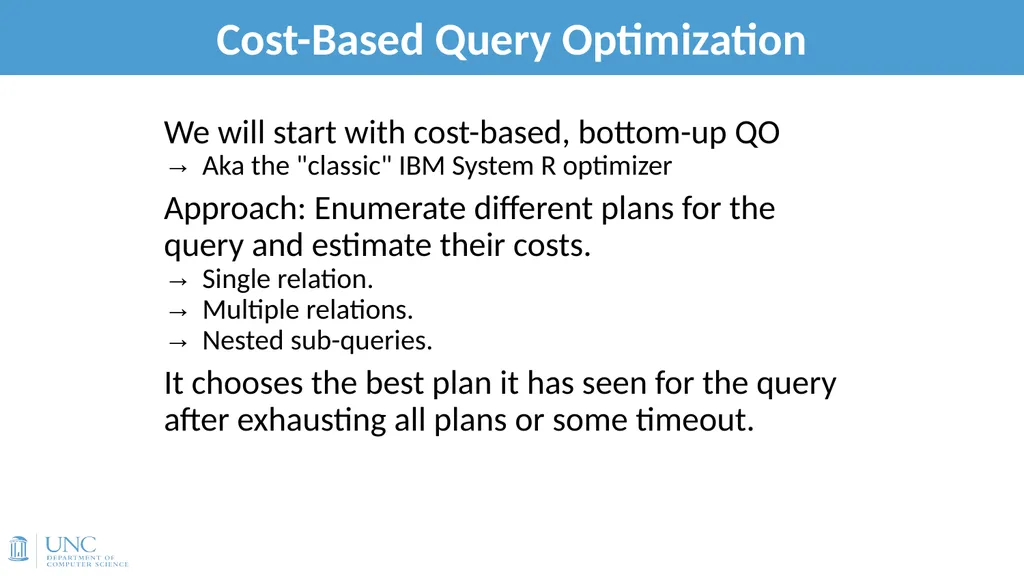
Cost-Based Query Optimization We will start with cost-based, bottom-up QO
Aka the "classic" IBM System R optimizer
Approach: Enumerate different plans for the query and estimate their costs.
Single relation.
Multiple relations.
Nested sub-queries.
It chooses the best plan it has seen for the query after exhausting all plans or some timeout. 19<br>
Aka the "classic" IBM System R optimizer
Approach: Enumerate different plans for the query and estimate their costs.
Single relation.
Multiple relations.
Nested sub-queries.
It chooses the best plan it has seen for the query after exhausting all plans or some timeout. 19<br>
20
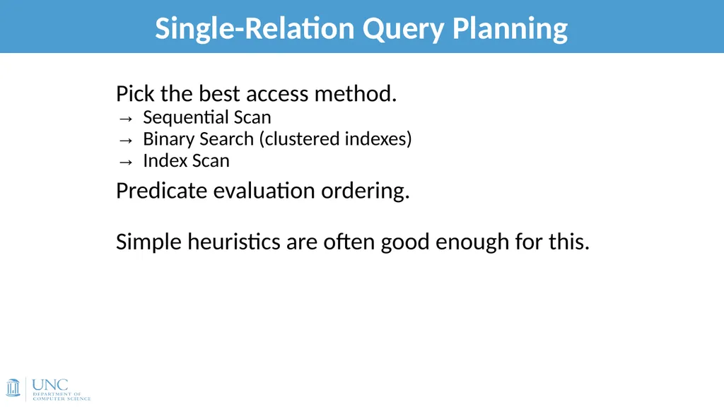
Single-Relation Query Planning Pick the best access method.
Sequential Scan
Binary Search (clustered indexes)
Index Scan
Predicate evaluation ordering.
Simple heuristics are often good enough for this. 20<br>
Sequential Scan
Binary Search (clustered indexes)
Index Scan
Predicate evaluation ordering.
Simple heuristics are often good enough for this. 20<br>
21
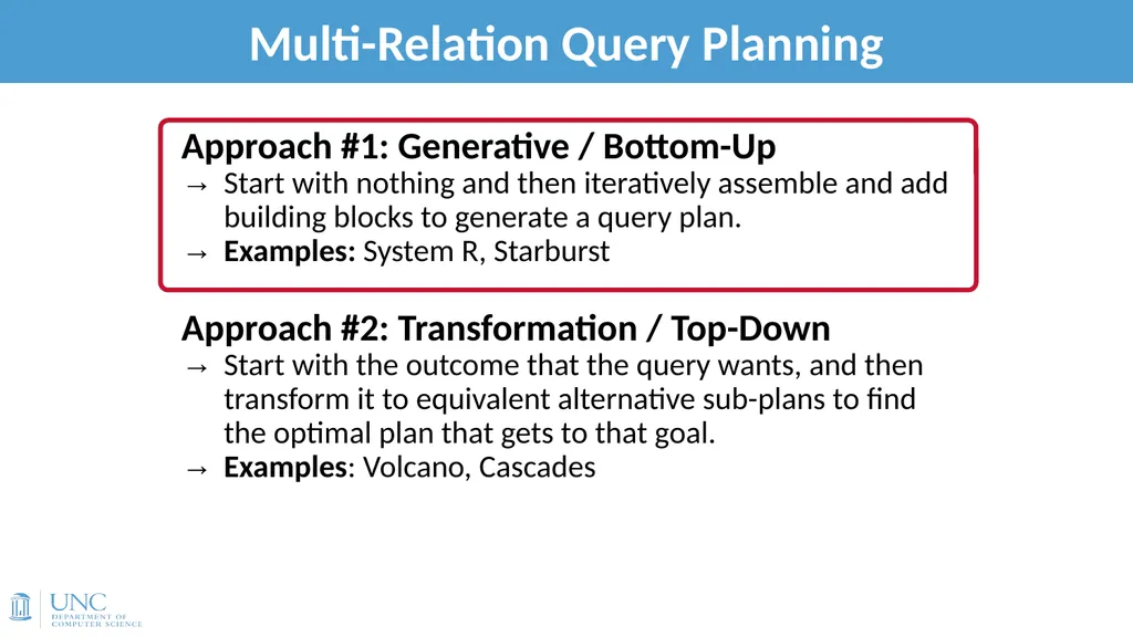
Multi-Relation Query Planning Approach #1: Generative / Bottom-Up
Start with nothing and then iteratively assemble and add building blocks to generate a query plan.
Examples: System R, Starburst
Approach #2: Transformation / Top-Down
Start with the outcome that the query wants, and then transform it to equivalent alternative sub-plans to find the optimal plan that gets to that goal.
Examples: Volcano, Cascades 21<br>
Start with nothing and then iteratively assemble and add building blocks to generate a query plan.
Examples: System R, Starburst
Approach #2: Transformation / Top-Down
Start with the outcome that the query wants, and then transform it to equivalent alternative sub-plans to find the optimal plan that gets to that goal.
Examples: Volcano, Cascades 21<br>
22
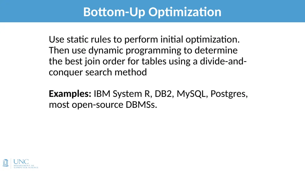
Bottom-Up Optimization Use static rules to perform initial optimization.
Then use dynamic programming to determine
the best join order for tables using a divide-and-conquer search method
Examples: IBM System R, DB2, MySQL, Postgres, most open-source DBMSs. 22<br>
Examples: IBM System R, DB2, MySQL, Postgres, most open-source DBMSs. 22<br>
23
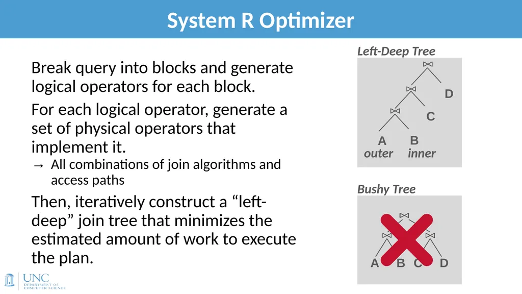
System R Optimizer Break query into blocks and generate logical operators for each block.
For each logical operator, generate a set of physical operators that implement it.
All combinations of join algorithms and access paths
Then, iteratively construct a “left-deep” join tree that minimizes the estimated amount of work to execute the plan. 23<br>
For each logical operator, generate a set of physical operators that implement it.
All combinations of join algorithms and access paths
Then, iteratively construct a “left-deep” join tree that minimizes the estimated amount of work to execute the plan. 23<br>
24
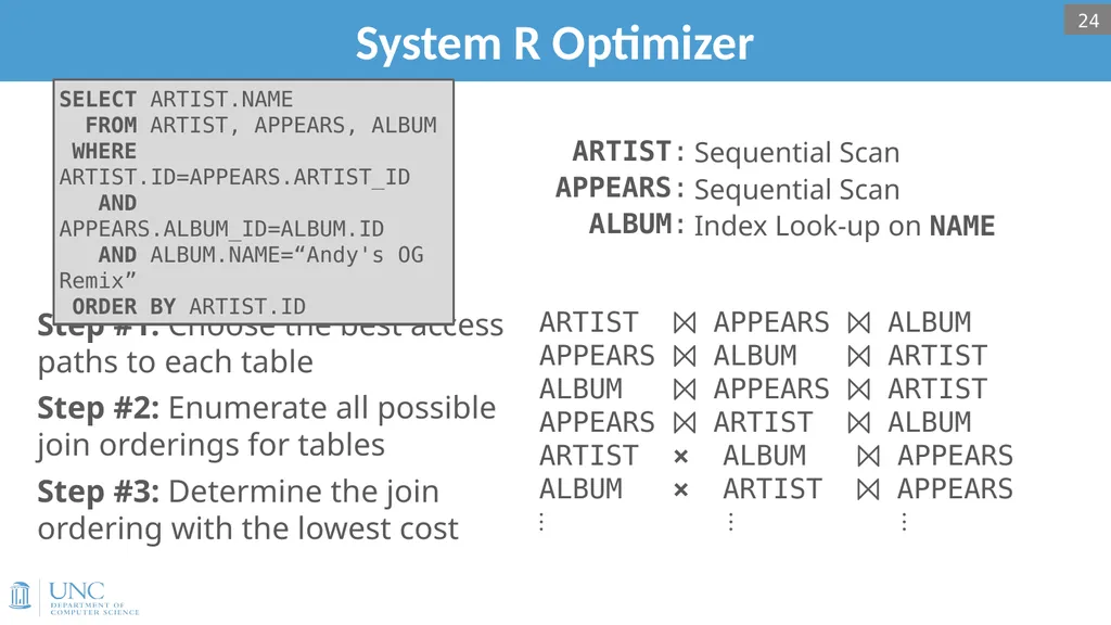
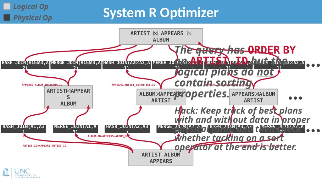
System R Optimizer 24 Step #1: Choose the best access paths to each table Step #3: Determine the join ordering with the lowest cost ARTIST ⨝ APPEARS ⨝ ALBUM
APPEARS ⨝ ALBUM ⨝ ARTIST
ALBUM ⨝ APPEARS ⨝ ARTIST
APPEARS ⨝ ARTIST ⨝ ALBUM
ARTIST × ALBUM ⨝ APPEARS
ALBUM × ARTIST ⨝ APPEARS
⋮ ⋮ ⋮ Step #2: Enumerate all possible join orderings for tables SELECT ARTIST.NAME
FROM ARTIST, APPEARS, ALBUM
WHERE ARTIST.ID=APPEARS.ARTIST_ID
AND APPEARS.ALBUM_ID=ALBUM.ID
AND ALBUM.NAME=“Andy's OG Remix”
ORDER BY ARTIST.ID<br>
APPEARS ⨝ ALBUM ⨝ ARTIST
ALBUM ⨝ APPEARS ⨝ ARTIST
APPEARS ⨝ ARTIST ⨝ ALBUM
ARTIST × ALBUM ⨝ APPEARS
ALBUM × ARTIST ⨝ APPEARS
⋮ ⋮ ⋮ Step #2: Enumerate all possible join orderings for tables SELECT ARTIST.NAME
FROM ARTIST, APPEARS, ALBUM
WHERE ARTIST.ID=APPEARS.ARTIST_ID
AND APPEARS.ALBUM_ID=ALBUM.ID
AND ALBUM.NAME=“Andy's OG Remix”
ORDER BY ARTIST.ID<br>
25
System R Optimizer 25 • • • • • • • • • ARTIST.ID=APPEARS.ARTIST_ID ALBUM.ID=APPEARS.ALBUM_ID APPEARS.ALBUM_ID=ALBUM.ID APPEARS.ALBUM_ID=ALBUM.ID APPEARS.ARTIST_ID=ARTIST.ID APPEARS.ARTIST_ID=ARTIST.ID The query has ORDER BY on ARTIST.ID but the logical plans do not contain sorting properties. Hack: Keep track of best plans with and without data in proper physical form, and then check whether tacking on a sort operator at the end is better.<br>
26
SYSTEM R OPTIMIZER 26<br>
27
Top-Down Optimization Start with a logical plan of what we want the query to be. Perform a branch-and-bound search to traverse the plan tree by converting logical operators into physical operators.
Keep track of global best plan during search.
Treat physical properties of data as first-class entities during planning.
Examples: MSSQL, Greenplum, CockroachDB 27<br>
Keep track of global best plan during search.
Treat physical properties of data as first-class entities during planning.
Examples: MSSQL, Greenplum, CockroachDB 27<br>
28
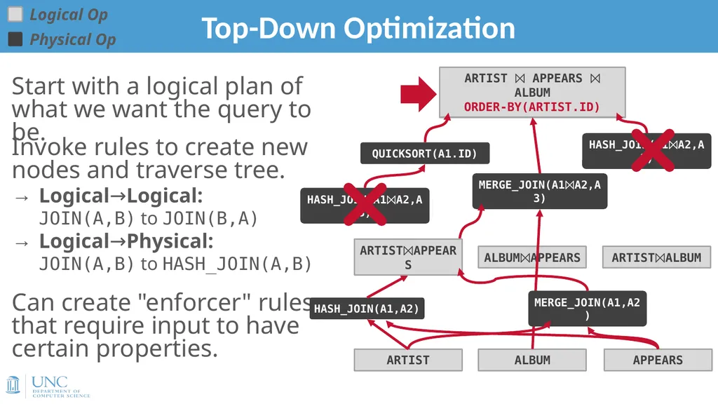
Top-Down Optimization 28 Invoke rules to create new nodes and traverse tree.
Logical→Logical: JOIN(A,B) to JOIN(B,A)
Logical→Physical: JOIN(A,B) to HASH_JOIN(A,B) Can create "enforcer" rules that require input to have certain properties. ARTIST ALBUM APPEARS ALBUM⨝APPEARS ARTIST⨝ALBUM Start with a logical plan of what we want the query to be.<br>
Logical→Logical: JOIN(A,B) to JOIN(B,A)
Logical→Physical: JOIN(A,B) to HASH_JOIN(A,B) Can create "enforcer" rules that require input to have certain properties. ARTIST ALBUM APPEARS ALBUM⨝APPEARS ARTIST⨝ALBUM Start with a logical plan of what we want the query to be.<br>
29
Observation Applications often execute nested queries.
We could optimize each block using the methods we have discussed.
However, this may be inefficient since we optimize each block separately without a global approach.
What if we could flatten a nested query into a single block and optimize it?
Then, apply single-block query optimization methods.
Even if one cannot flatten to a single block, flattening to fewer blocks is still beneficial. 29<br>
We could optimize each block using the methods we have discussed.
However, this may be inefficient since we optimize each block separately without a global approach.
What if we could flatten a nested query into a single block and optimize it?
Then, apply single-block query optimization methods.
Even if one cannot flatten to a single block, flattening to fewer blocks is still beneficial. 29<br>
30
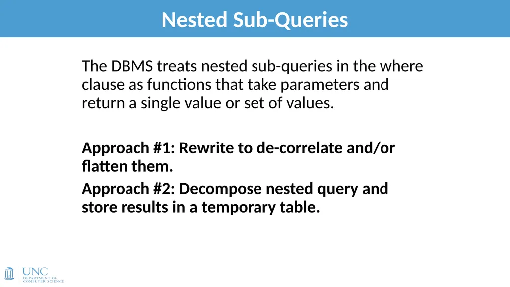
Nested Sub-Queries The DBMS treats nested sub-queries in the where clause as functions that take parameters and return a single value or set of values.
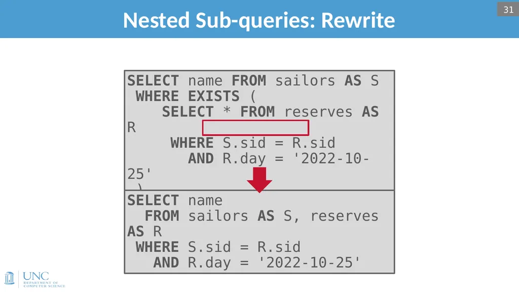
Approach #1: Rewrite to de-correlate and/or flatten them.
Approach #2: Decompose nested query and store results in a temporary table. 30<br>
Approach #1: Rewrite to de-correlate and/or flatten them.
Approach #2: Decompose nested query and store results in a temporary table. 30<br>
31
Nested Sub-queries: Rewrite 31 SELECT name FROM sailors AS S
WHERE EXISTS (
SELECT * FROM reserves AS R
WHERE S.sid = R.sid
AND R.day = '2022-10-25'
) SELECT name
FROM sailors AS S, reserves AS R
WHERE S.sid = R.sid
AND R.day = '2022-10-25'<br>
WHERE EXISTS (
SELECT * FROM reserves AS R
WHERE S.sid = R.sid
AND R.day = '2022-10-25'
) SELECT name
FROM sailors AS S, reserves AS R
WHERE S.sid = R.sid
AND R.day = '2022-10-25'<br>
32
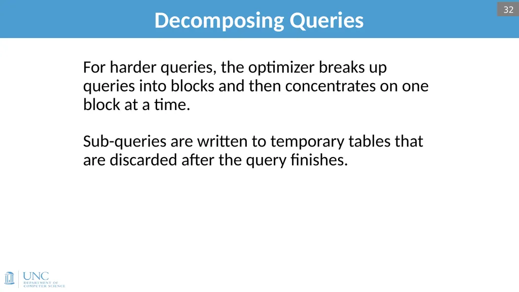
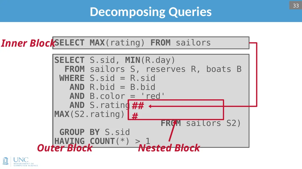
Decomposing Queries For harder queries, the optimizer breaks up queries into blocks and then concentrates on one block at a time.
Sub-queries are written to temporary tables that are discarded after the query finishes. 32<br>
Sub-queries are written to temporary tables that are discarded after the query finishes. 32<br>
33
Decomposing Queries 33 SELECT S.sid, MIN(R.day)
FROM sailors S, reserves R, boats B
WHERE S.sid = R.sid
AND R.bid = B.bid
AND B.color = 'red'
AND S.rating = (SELECT MAX(S2.rating)
FROM sailors S2)
GROUP BY S.sid
HAVING COUNT(*) > 1 Nested Block Outer Block SELECT MAX(rating) FROM sailors Inner Block<br>
FROM sailors S, reserves R, boats B
WHERE S.sid = R.sid
AND R.bid = B.bid
AND B.color = 'red'
AND S.rating = (SELECT MAX(S2.rating)
FROM sailors S2)
GROUP BY S.sid
HAVING COUNT(*) > 1 Nested Block Outer Block SELECT MAX(rating) FROM sailors Inner Block<br>
34
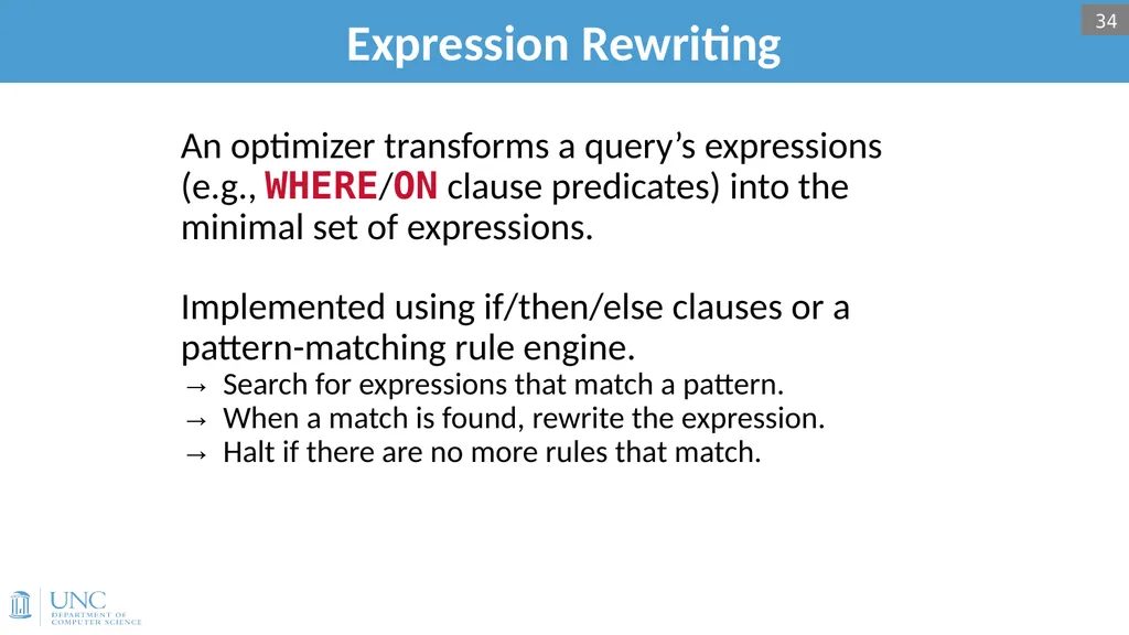
Expression Rewriting An optimizer transforms a query’s expressions (e.g., WHERE/ON clause predicates) into the minimal set of expressions.
Implemented using if/then/else clauses or a pattern-matching rule engine.
Search for expressions that match a pattern.
When a match is found, rewrite the expression.
Halt if there are no more rules that match. 34<br>
Implemented using if/then/else clauses or a pattern-matching rule engine.
Search for expressions that match a pattern.
When a match is found, rewrite the expression.
Halt if there are no more rules that match. 34<br>
35
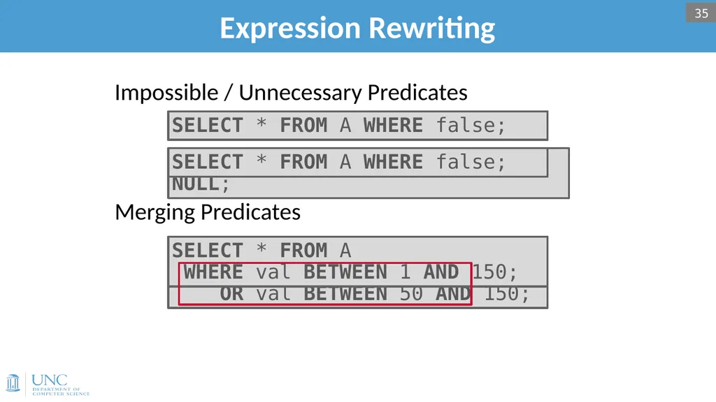
Expression Rewriting Impossible / Unnecessary Predicates
Merging Predicates 35 SELECT * FROM A WHERE 1 = 0; SELECT * FROM A WHERE NOW() IS NULL; SELECT * FROM A WHERE val BETWEEN 1 AND 100 OR val BETWEEN 50 AND 150; SELECT * FROM A WHERE val BETWEEN 1 AND 150; SELECT * FROM A WHERE false; SELECT * FROM A WHERE RANDOM() IS NULL; SELECT * FROM A WHERE false;<br>
Merging Predicates 35 SELECT * FROM A WHERE 1 = 0; SELECT * FROM A WHERE NOW() IS NULL; SELECT * FROM A WHERE val BETWEEN 1 AND 100 OR val BETWEEN 50 AND 150; SELECT * FROM A WHERE val BETWEEN 1 AND 150; SELECT * FROM A WHERE false; SELECT * FROM A WHERE RANDOM() IS NULL; SELECT * FROM A WHERE false;<br>
36
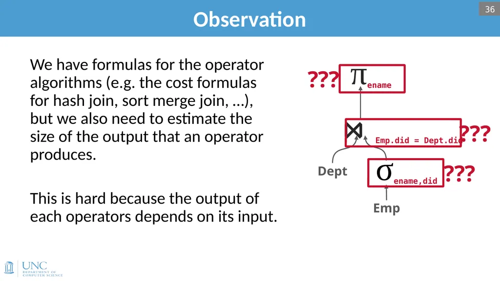
Observation We have formulas for the operator algorithms (e.g. the cost formulas for hash join, sort merge join, …), but we also need to estimate the size of the output that an operator produces.
This is hard because the output of each operators depends on its input. 36<br>
This is hard because the output of each operators depends on its input. 36<br>
37
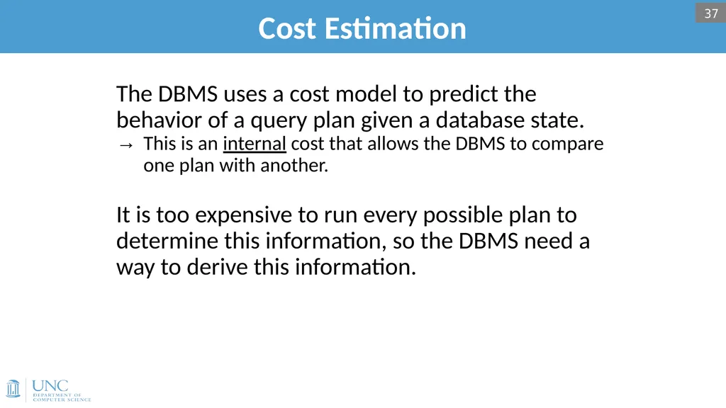
Cost Estimation The DBMS uses a cost model to predict the behavior of a query plan given a database state.
This is an internal cost that allows the DBMS to compare one plan with another.
It is too expensive to run every possible plan to determine this information, so the DBMS need a way to derive this information. 37<br>
This is an internal cost that allows the DBMS to compare one plan with another.
It is too expensive to run every possible plan to determine this information, so the DBMS need a way to derive this information. 37<br>
38
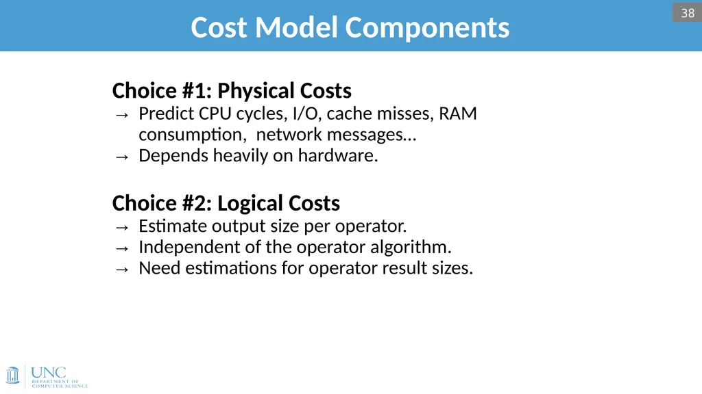
Cost Model Components Choice #1: Physical Costs
Predict CPU cycles, I/O, cache misses, RAM consumption, network messages…
Depends heavily on hardware.
Choice #2: Logical Costs
Estimate output size per operator.
Independent of the operator algorithm.
Need estimations for operator result sizes. 38<br>
Predict CPU cycles, I/O, cache misses, RAM consumption, network messages…
Depends heavily on hardware.
Choice #2: Logical Costs
Estimate output size per operator.
Independent of the operator algorithm.
Need estimations for operator result sizes. 38<br>
39
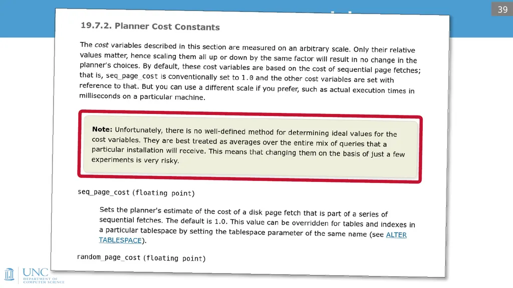
Postgres Cost Model Uses a combination of CPU and I/O costs that are weighted by “magic” constant factors.
Default settings are obviously for a disk-resident database without a lot of memory:
Processing a tuple in memory is 400x faster than reading a tuple from disk.
Sequential I/O is 4x faster than random I/O. 39<br>
Default settings are obviously for a disk-resident database without a lot of memory:
Processing a tuple in memory is 400x faster than reading a tuple from disk.
Sequential I/O is 4x faster than random I/O. 39<br>
40
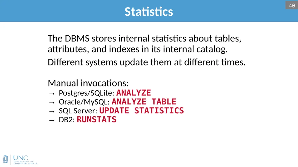
Statistics The DBMS stores internal statistics about tables, attributes, and indexes in its internal catalog.
Different systems update them at different times.
Manual invocations:
Postgres/SQLite: ANALYZE
Oracle/MySQL: ANALYZE TABLE
SQL Server: UPDATE STATISTICS
DB2: RUNSTATS 40<br>
Different systems update them at different times.
Manual invocations:
Postgres/SQLite: ANALYZE
Oracle/MySQL: ANALYZE TABLE
SQL Server: UPDATE STATISTICS
DB2: RUNSTATS 40<br>
41
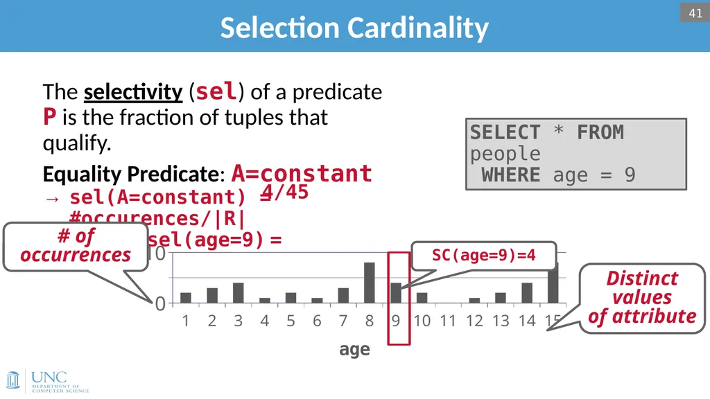
Selection Cardinality The selectivity (sel) of a predicate P is the fraction of tuples that qualify.
Equality Predicate: A=constant
sel(A=constant) = #occurences/|R|
Example: sel(age=9) = 41 SC(age=9)=4 SELECT * FROM people WHERE age = 9 4/45 Distinct values of attribute # of occurrences<br>
Equality Predicate: A=constant
sel(A=constant) = #occurences/|R|
Example: sel(age=9) = 41 SC(age=9)=4 SELECT * FROM people WHERE age = 9 4/45 Distinct values of attribute # of occurrences<br>
42
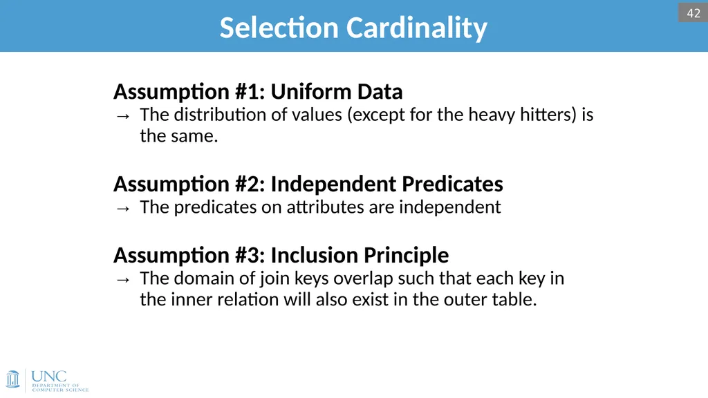
Selection Cardinality Assumption #1: Uniform Data
The distribution of values (except for the heavy hitters) is the same.
Assumption #2: Independent Predicates
The predicates on attributes are independent
Assumption #3: Inclusion Principle
The domain of join keys overlap such that each key in the inner relation will also exist in the outer table. 42<br>
The distribution of values (except for the heavy hitters) is the same.
Assumption #2: Independent Predicates
The predicates on attributes are independent
Assumption #3: Inclusion Principle
The domain of join keys overlap such that each key in the inner relation will also exist in the outer table. 42<br>
43
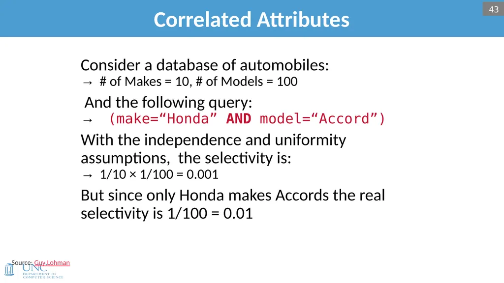
Correlated Attributes Consider a database of automobiles:
# of Makes = 10, # of Models = 100
And the following query:
(make=“Honda” AND model=“Accord”)
With the independence and uniformity assumptions, the selectivity is:
1/10 × 1/100 = 0.001
But since only Honda makes Accords the real selectivity is 1/100 = 0.01 43 Source: Guy Lohman<br>
# of Makes = 10, # of Models = 100
And the following query:
(make=“Honda” AND model=“Accord”)
With the independence and uniformity assumptions, the selectivity is:
1/10 × 1/100 = 0.001
But since only Honda makes Accords the real selectivity is 1/100 = 0.01 43 Source: Guy Lohman<br>
44
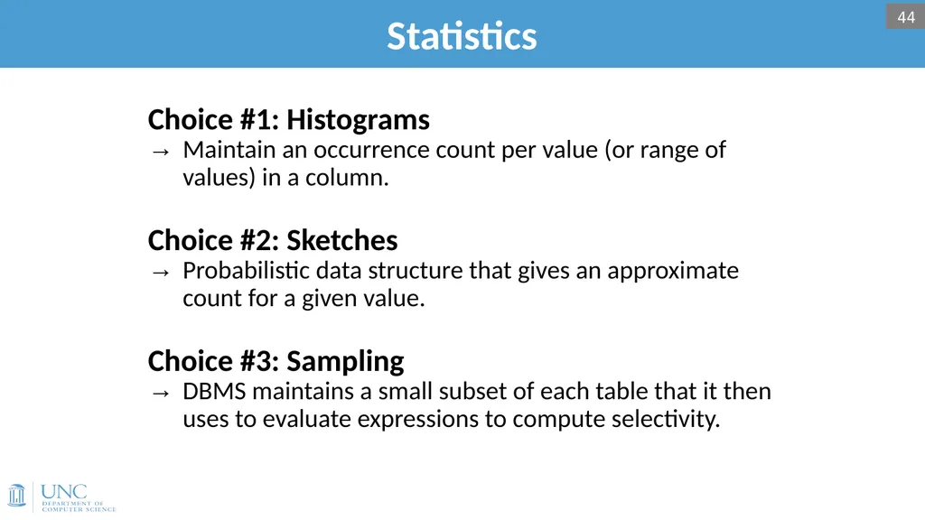
Statistics Choice #1: Histograms
Maintain an occurrence count per value (or range of values) in a column.
Choice #2: Sketches
Probabilistic data structure that gives an approximate count for a given value.
Choice #3: Sampling
DBMS maintains a small subset of each table that it then uses to evaluate expressions to compute selectivity. 44<br>
Maintain an occurrence count per value (or range of values) in a column.
Choice #2: Sketches
Probabilistic data structure that gives an approximate count for a given value.
Choice #3: Sampling
DBMS maintains a small subset of each table that it then uses to evaluate expressions to compute selectivity. 44<br>
45
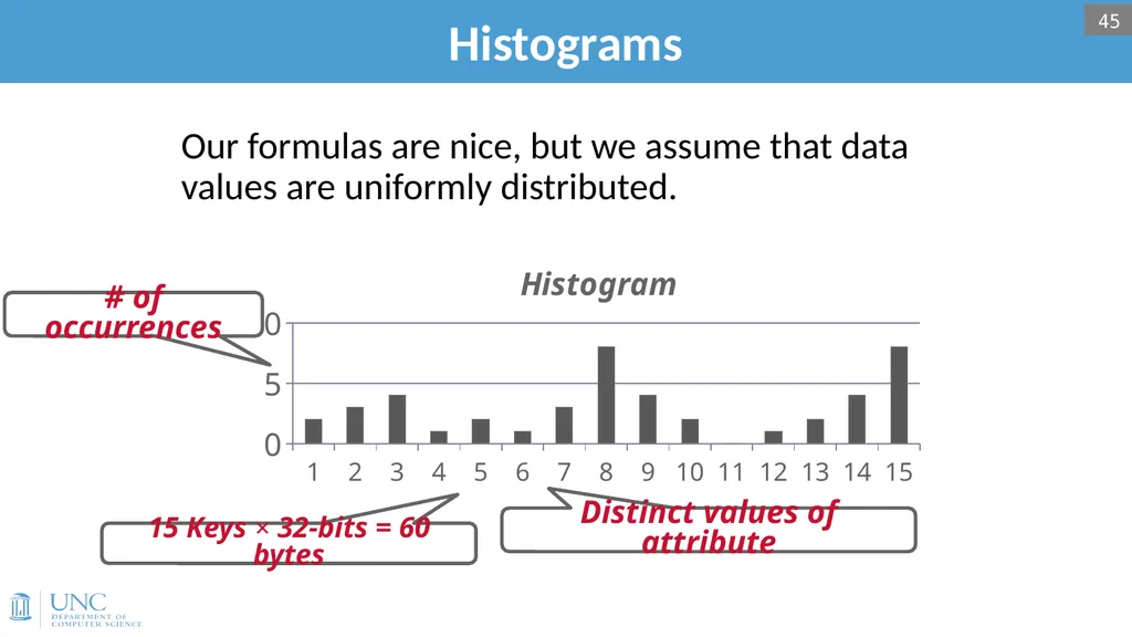
Histograms Our formulas are nice, but we assume that data values are uniformly distributed. 45 15 Keys × 32-bits = 60 bytes Distinct values of attribute # of occurrences<br>
46
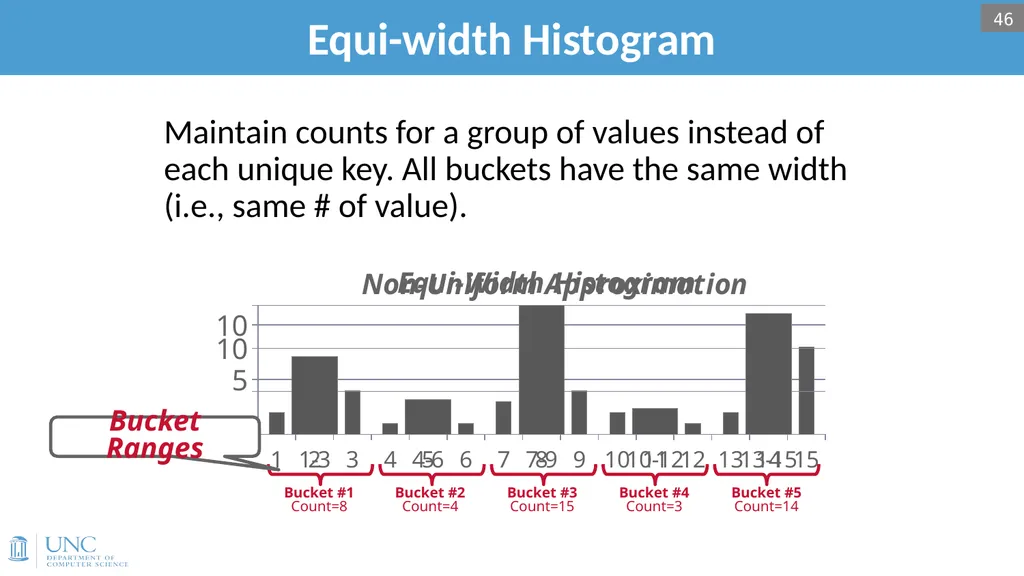
Equi-width Histogram Maintain counts for a group of values instead of each unique key. All buckets have the same width (i.e., same # of value). 46 Bucket Ranges<br>
47
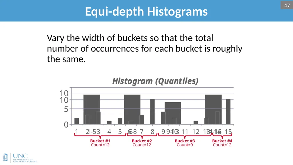
Equi-depth Histograms Vary the width of buckets so that the total number of occurrences for each bucket is roughly the same. 47<br>
48
Sketches Probabilistic data structures that generate approximate statistics about a data set.
Cost-model can replace histograms with sketches to improve its selectivity estimate accuracy.
Most common examples:
Count-Min Sketch (1988): Approximate frequency count of elements in a set.
HyperLogLog (2007): Approximate the number of distinct elements in a set. 48<br>
Cost-model can replace histograms with sketches to improve its selectivity estimate accuracy.
Most common examples:
Count-Min Sketch (1988): Approximate frequency count of elements in a set.
HyperLogLog (2007): Approximate the number of distinct elements in a set. 48<br>
49
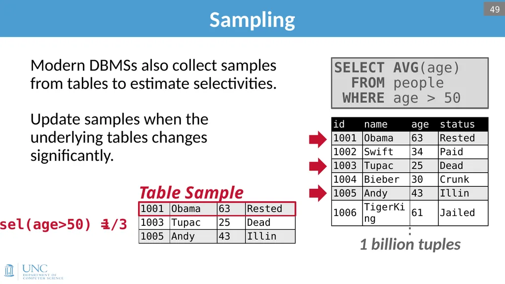
Sampling Modern DBMSs also collect samples from tables to estimate selectivities.
Update samples when the underlying tables changes significantly. 49 ⋮
1 billion tuples 1/3 sel(age>50) = SELECT AVG(age) FROM people WHERE age > 50 Table Sample<br>
Update samples when the underlying tables changes significantly. 49 ⋮
1 billion tuples 1/3 sel(age>50) = SELECT AVG(age) FROM people WHERE age > 50 Table Sample<br>
50
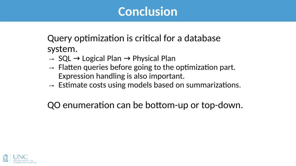
Conclusion Query optimization is critical for a database system.
SQL → Logical Plan → Physical Plan
Flatten queries before going to the optimization part. Expression handling is also important.
Estimate costs using models based on summarizations.
QO enumeration can be bottom-up or top-down. 50<br>
SQL → Logical Plan → Physical Plan
Flatten queries before going to the optimization part. Expression handling is also important.
Estimate costs using models based on summarizations.
QO enumeration can be bottom-up or top-down. 50<br>
51
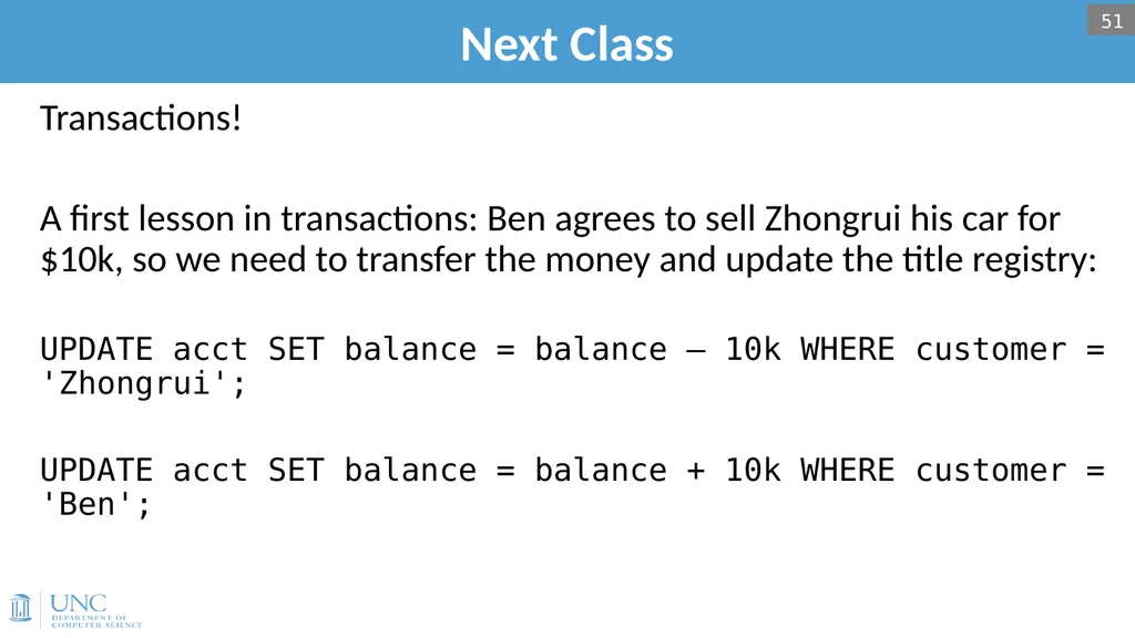
Next Class Transactions!
A first lesson in transactions: Ben agrees to sell Zhongrui his car for $10k, so we need to transfer the money and update the title registry:
UPDATE acct SET balance = balance – 10k WHERE customer = 'Zhongrui';
UPDATE acct SET balance = balance + 10k WHERE customer = 'Ben'; 51<br>
A first lesson in transactions: Ben agrees to sell Zhongrui his car for $10k, so we need to transfer the money and update the title registry:
UPDATE acct SET balance = balance – 10k WHERE customer = 'Zhongrui';
UPDATE acct SET balance = balance + 10k WHERE customer = 'Ben'; 51<br>
52
Essential Query Optimization papers 52 Surajit Chaudhuri: An Overview of Query Optimization in Relational Systems. PODS 1998: 34-43 Goetz Graefe, William J. McKenna: The Volcano Optimizer Generator: Extensibility and Efficient Search. ICDE 1993: 209-218 Patricia G. Selinger, Morton M. Astrahan, Donald D. Chamberlin, Raymond A. Lorie, Thomas G. Price: Access Path Selection in a Relational Database Management System. SIGMOD Conference 1979: 23-34 Umeshwar Dayal: Of Nests and Trees: A Unified Approach to Processing Queries That Contain Nested Subqueries, Aggregates, and Quantifiers. VLDB 1987: 197-208 Bonus<br>
53
Suggestions if you are going to build a QO Rule 1: Read lots of papers, especially from the 80s & 90s.
Expect new combinations, only partially new core inventions.
Rule 2: Early on, test various workloads on the QO.
QOs harden over time as they “see” new workloads. Let them see more ASAP.
Rule 3: Throw away the initial one (or two) and start anew.
The hard part is going to be nitty-gritty details like data structures and pointers to shared objects; e.g., the list of predicates and the query graph structure, … You will NOT get this right in the first pass. Don’t try to patch; be prepared to rewrite. 53 Bonus<br>
Expect new combinations, only partially new core inventions.
Rule 2: Early on, test various workloads on the QO.
QOs harden over time as they “see” new workloads. Let them see more ASAP.
Rule 3: Throw away the initial one (or two) and start anew.
The hard part is going to be nitty-gritty details like data structures and pointers to shared objects; e.g., the list of predicates and the query graph structure, … You will NOT get this right in the first pass. Don’t try to patch; be prepared to rewrite. 53 Bonus<br>
54
RELATIONAL ALGEBRA EQUIVALENCES Two relational algebra expressions are equivalent if they generate the same set of tuples.
The DBMS can identify better query plans without a cost model.
This is often called query rewriting. 54<br>
The DBMS can identify better query plans without a cost model.
This is often called query rewriting. 54<br>
55
PREDICATE PUSHDOWN 55 SELECT s.name, e.cid
FROM student AS s JOIN enrolled AS e
ON s.sid = e.sid
WHERE e.grade = 'A' πname, cid(σgrade='A'(student⋈enrolled))<br>
FROM student AS s JOIN enrolled AS e
ON s.sid = e.sid
WHERE e.grade = 'A' πname, cid(σgrade='A'(student⋈enrolled))<br>
56
RELATIONAL ALGEBRA EQUIVALENCES 56 πname, cid(σgrade='A'(student⋈enrolled)) πname, cid(student⋈(σgrade='A'(enrolled))) = SELECT s.name, e.cid
FROM student AS s JOIN enrolled AS e
ON s.sid = e.sid
WHERE e.grade = 'A'<br>
FROM student AS s JOIN enrolled AS e
ON s.sid = e.sid
WHERE e.grade = 'A'<br>
57
RELATIONAL ALGEBRA EQUIVALENCES Selections:
Perform filters as early as possible.
Break a complex predicate, and push down σp1∧p2∧…pn(R) = σp1(σp2(…σpn(R)))
Simplify a complex predicate
(X=Y AND Y=3) → X=3 AND Y=3 57<br>
Perform filters as early as possible.
Break a complex predicate, and push down σp1∧p2∧…pn(R) = σp1(σp2(…σpn(R)))
Simplify a complex predicate
(X=Y AND Y=3) → X=3 AND Y=3 57<br>
58
RELATIONAL ALGEBRA EQUIVALENCES Joins:
Commutative, associative R⋈S = S⋈R (R⋈S)⋈T = R⋈(S⋈T)
The number of different join orderings for an n-way join is a Catalan Number (≈4n)
Exhaustive enumeration will be too slow. 58<br>
Commutative, associative R⋈S = S⋈R (R⋈S)⋈T = R⋈(S⋈T)
The number of different join orderings for an n-way join is a Catalan Number (≈4n)
Exhaustive enumeration will be too slow. 58<br>
59
RELATIONAL ALGEBRA EQUIVALENCES Projections:
Perform them early to create smaller tuples and reduce intermediate results (if duplicates are eliminated)
Project out all attributes except the ones requested or required (e.g., joining keys)
This is not important for a column store… 59<br>
Perform them early to create smaller tuples and reduce intermediate results (if duplicates are eliminated)
Project out all attributes except the ones requested or required (e.g., joining keys)
This is not important for a column store… 59<br>
60
PROJECTION PUSHDOWN 60 SELECT s.name, e.cid
FROM student AS s JOIN enrolled AS e
ON s.sid = e.sid
WHERE e.grade = 'A'<br>
FROM student AS s JOIN enrolled AS e
ON s.sid = e.sid
WHERE e.grade = 'A'<br>
61
STATISTICS For each relation R, the DBMS maintains the following information:
NR: Number of tuples in R.
V(A,R): Number of distinct values for attribute A. 61<br>
NR: Number of tuples in R.
V(A,R): Number of distinct values for attribute A. 61<br>
62
DERIVABLE STATISTICS The selection cardinality SC(A,R) is the average number of records with a value for an attribute A given NR / V(A,R)
Note that this formula assumes data uniformity where every value has the same frequency as all other values.
Example: 10,000 students, 10 colleges – how many students in SCS? 62<br>
Note that this formula assumes data uniformity where every value has the same frequency as all other values.
Example: 10,000 students, 10 colleges – how many students in SCS? 62<br>
63
LOGICAL COSTS Equality predicates on unique keys are easy to estimate.
Computing the logical cost of complex predicates is more difficult… 63 SELECT * FROM people WHERE id = 123 SELECT * FROM people WHERE val > 1000 SELECT * FROM people WHERE age = 30 AND status = 'Lit'
AND age+id IN (1,2,3) CREATE TABLE people (
id INT PRIMARY KEY,
val INT NOT NULL,
age INT NOT NULL,
status VARCHAR(16)
);<br>
Computing the logical cost of complex predicates is more difficult… 63 SELECT * FROM people WHERE id = 123 SELECT * FROM people WHERE val > 1000 SELECT * FROM people WHERE age = 30 AND status = 'Lit'
AND age+id IN (1,2,3) CREATE TABLE people (
id INT PRIMARY KEY,
val INT NOT NULL,
age INT NOT NULL,
status VARCHAR(16)
);<br>
64
SELECTIONS – COMPLEX PREDICATES Range Predicate:
sel(A>=a) = (Amax– a+1) / (Amax– Amin+1)
Example: sel(age>=2) 64 ≈ (4–2+1) / (4–0+1)
≈ 3/5 agemin = 0 SELECT * FROM people WHERE age >= 2 agemax = 4<br>
sel(A>=a) = (Amax– a+1) / (Amax– Amin+1)
Example: sel(age>=2) 64 ≈ (4–2+1) / (4–0+1)
≈ 3/5 agemin = 0 SELECT * FROM people WHERE age >= 2 agemax = 4<br>
65
SELECTIONS – COMPLEX PREDICATES Negation Query:
sel(not P) = 1 – sel(P)
Example: sel(age != 2)
Observation: Selectivity ≈ Probability 65 = 1 – (1/5) = 4/5 SC(age=2)=1 SC(age!=2)=2 SC(age!=2)=2 SELECT * FROM people WHERE age != 2<br>
sel(not P) = 1 – sel(P)
Example: sel(age != 2)
Observation: Selectivity ≈ Probability 65 = 1 – (1/5) = 4/5 SC(age=2)=1 SC(age!=2)=2 SC(age!=2)=2 SELECT * FROM people WHERE age != 2<br>
66
SELECTIONS – COMPLEX PREDICATES Conjunction:
sel(P1 ⋀ P2) = sel(P1) ∙ sel(P2)
sel(age=2 ⋀ name LIKE 'A%')
This assumes that the predicates are independent. 66 Not always true in practice! SELECT * FROM people WHERE age = 2
AND name LIKE 'A%' P1 P2<br>
sel(P1 ⋀ P2) = sel(P1) ∙ sel(P2)
sel(age=2 ⋀ name LIKE 'A%')
This assumes that the predicates are independent. 66 Not always true in practice! SELECT * FROM people WHERE age = 2
AND name LIKE 'A%' P1 P2<br>
67
SELECTIONS – COMPLEX PREDICATES Disjunction:
sel(P1 ⋁ P2) = sel(P1) + sel(P2) – sel(P1⋀P2) = sel(P1) + sel(P2) – sel(P1) ∙ sel(P2)
sel(age=2 OR name LIKE 'A%')
This again assumes that the selectivities are independent. 67 SELECT * FROM people WHERE age = 2
OR name LIKE 'A%' P1 P2<br>
sel(P1 ⋁ P2) = sel(P1) + sel(P2) – sel(P1⋀P2) = sel(P1) + sel(P2) – sel(P1) ∙ sel(P2)
sel(age=2 OR name LIKE 'A%')
This again assumes that the selectivities are independent. 67 SELECT * FROM people WHERE age = 2
OR name LIKE 'A%' P1 P2<br>
68
RESULT SIZE ESTIMATION FOR JOINS Given a join of R and S, what is the range of possible result sizes in # of tuples?
In other words, for a given tuple of R, how many tuples of S will it match?
Assume each key in the inner relation will exist in the outer table.
This is super hard. 68<br>
In other words, for a given tuple of R, how many tuples of S will it match?
Assume each key in the inner relation will exist in the outer table.
This is super hard. 68<br>
69
RESULT SIZE ESTIMATION FOR JOINS General case: Rcols⋂Scols={A} where A is not a primary key for either table.
Match each R-tuple with S-tuples: estSize ≈ NR ∙ NS / V(A,S)
Symmetrically, for S: estSize ≈ NR ∙ NS / V(A,R)
Overall:
estSize ≈ NR ∙ NS / max({V(A,S), V(A,R)}) 69<br>
Match each R-tuple with S-tuples: estSize ≈ NR ∙ NS / V(A,S)
Symmetrically, for S: estSize ≈ NR ∙ NS / V(A,R)
Overall:
estSize ≈ NR ∙ NS / max({V(A,S), V(A,R)}) 69<br>
70
LOGICAL PLAN OPTIMIZATION Transform a logical plan into an equivalent logical plan using pattern matching rules.
The goal is to increase the likelihood of enumerating the optimal plan in the search.
Cannot compare plans because there is no cost model but can "direct" a transformation to a preferred side. 70<br>
The goal is to increase the likelihood of enumerating the optimal plan in the search.
Cannot compare plans because there is no cost model but can "direct" a transformation to a preferred side. 70<br>
71
LOGICAL QUERY OPTIMIZATION Split Conjunctive Predicates
Predicate Pushdown
Replace Cartesian Products with Joins
Projection Pushdown 71 Source: Thomas Neumann<br>
Predicate Pushdown
Replace Cartesian Products with Joins
Projection Pushdown 71 Source: Thomas Neumann<br>
72
SPLIT CONJUNCTIVE PREDICATES 72 SELECT ARTIST.NAME
FROM ARTIST, APPEARS, ALBUM
WHERE ARTIST.ID=APPEARS.ARTIST_ID
AND APPEARS.ALBUM_ID=ALBUM.ID
AND ALBUM.NAME="Andy's OG Remix" ARTIST APPEARS ALBUM Decompose predicates into their simplest forms to make it easier for the optimizer to move them around.<br>
FROM ARTIST, APPEARS, ALBUM
WHERE ARTIST.ID=APPEARS.ARTIST_ID
AND APPEARS.ALBUM_ID=ALBUM.ID
AND ALBUM.NAME="Andy's OG Remix" ARTIST APPEARS ALBUM Decompose predicates into their simplest forms to make it easier for the optimizer to move them around.<br>
73
SELECTION CARDINALITY Formula depends on type of predicate:
Equality
Range
Negation
Conjunction
Disjunction 73 Selection Cardinality # of tuples sel(P) = SC(P) / NR<br>
Equality
Range
Negation
Conjunction
Disjunction 73 Selection Cardinality # of tuples sel(P) = SC(P) / NR<br>
74
EXPRESSION REWRITING Join Elimination with Sub-Query 74 SELECT * FROM A AS A1
WHERE EXISTS(SELECT val FROM A AS A2
WHERE A1.id = A2.id); SELECT * FROM A; Source: Lukas Eder CREATE TABLE A (
id INT PRIMARY KEY,
val INT NOT NULL );<br>
WHERE EXISTS(SELECT val FROM A AS A2
WHERE A1.id = A2.id); SELECT * FROM A; Source: Lukas Eder CREATE TABLE A (
id INT PRIMARY KEY,
val INT NOT NULL );<br>
75
IBM DB2 COST MODEL Database characteristics in system catalogs
Hardware environment (microbenchmarks)
Storage device characteristics (microbenchmarks)
Communications bandwidth (distributed only)
Memory resources (buffer pools, sort heaps)
Concurrency Environment
Average number of users
Isolation level / blocking
Number of available locks 75 Source: Guy Lohman<br>
Hardware environment (microbenchmarks)
Storage device characteristics (microbenchmarks)
Communications bandwidth (distributed only)
Memory resources (buffer pools, sort heaps)
Concurrency Environment
Average number of users
Isolation level / blocking
Number of available locks 75 Source: Guy Lohman<br>