
Lesson #18 MAT 1372 Statistics with Probability
Description: Lesson 18 MAT 1372 Statistics with Probability The Central Limit Theorem If samples of size n 30 are drawn from any population with mean µ and standard deviation σ, then the sampling distribution of sample means approximates a normal
Related Topics
Download Presentation
"Lesson #18 MAT 1372 Statistics with Probability" is the property of its rightful owner. Permission is granted to download and print the materials on this website for personal, non-commercial use only, and to display it on your personal computer provided you do not modify the materials and that you retain all copyright notices contained in the materials. By downloading content from our website, you accept the terms of this agreement.
Presentation Transcript
slide1. Lesson #18 MAT 1372 Statistics with Probability<br>
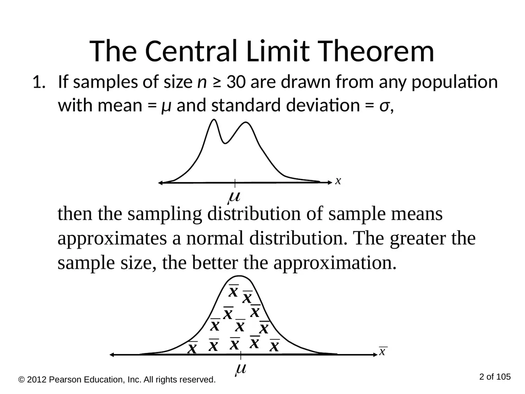
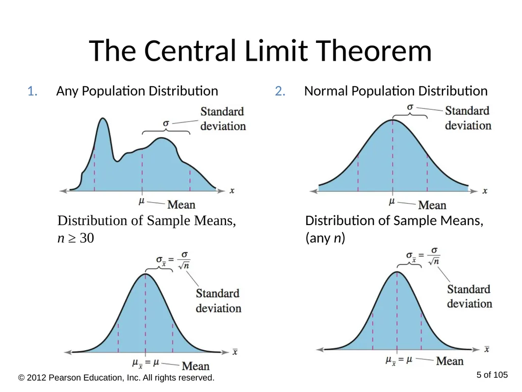
slide2. The Central Limit Theorem If samples of size n ≥ 30 are drawn from any population with mean = µ and standard deviation = σ, then the sampling distribution of sample means approximates a normal distribution. The greater the sample size, the better the approximation. © 2012 Pearson Education, Inc. All rights reserved. 2 of 105<br>
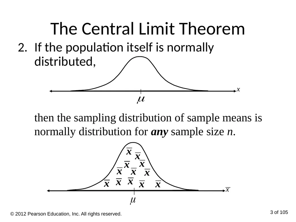
slide3. The Central Limit Theorem If the population itself is normally distributed, then the sampling distribution of sample means is normally distribution for any sample size n. © 2012 Pearson Education, Inc. All rights reserved. 3 of 105<br>
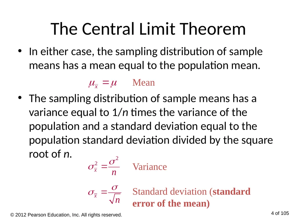
slide4. The Central Limit Theorem In either case, the sampling distribution of sample means has a mean equal to the population mean.
The sampling distribution of sample means has a variance equal to 1/n times the variance of the population and a standard deviation equal to the population standard deviation divided by the square root of n. Variance Standard deviation (standard error of the mean) © 2012 Pearson Education, Inc. All rights reserved. 4 of 105 Mean<br>
slide5. The Central Limit Theorem Any Population Distribution Normal Population Distribution Distribution of Sample Means, n ≥ 30 Distribution of Sample Means, (any n) © 2012 Pearson Education, Inc. All rights reserved. 5 of 105<br>
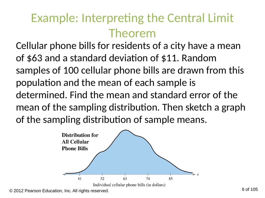
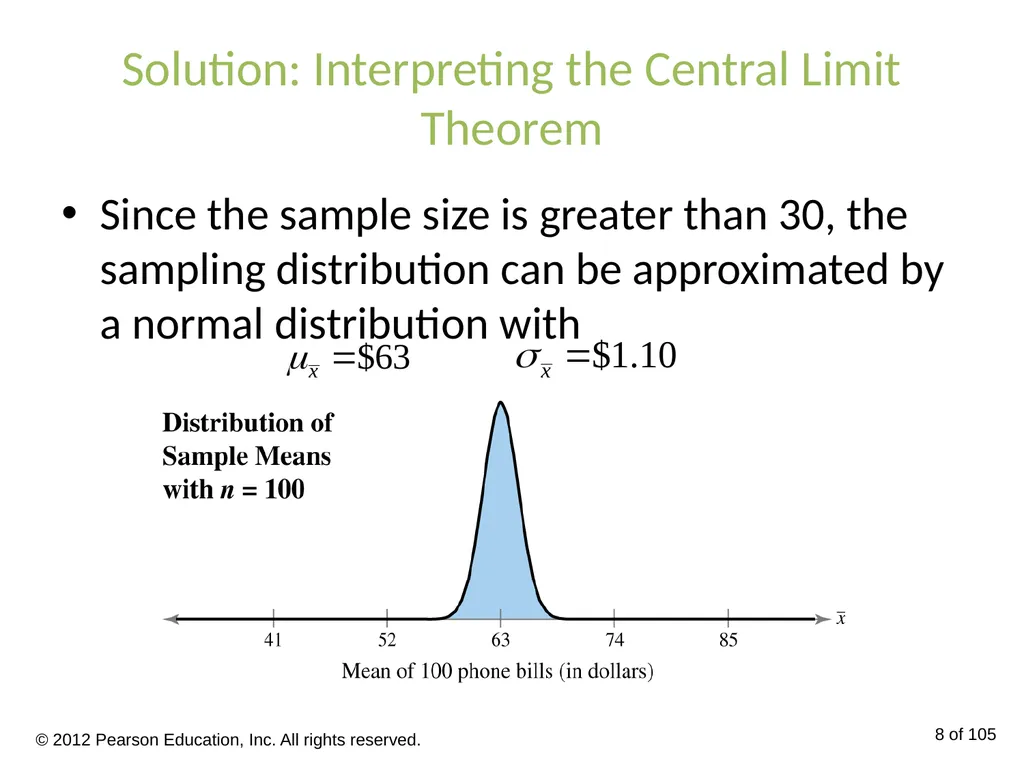
slide6. Example: Interpreting the Central Limit Theorem Cellular phone bills for residents of a city have a mean of $63 and a standard deviation of $11. Random samples of 100 cellular phone bills are drawn from this population and the mean of each sample is determined. Find the mean and standard error of the mean of the sampling distribution. Then sketch a graph of the sampling distribution of sample means. © 2012 Pearson Education, Inc. All rights reserved. 6 of 105<br>
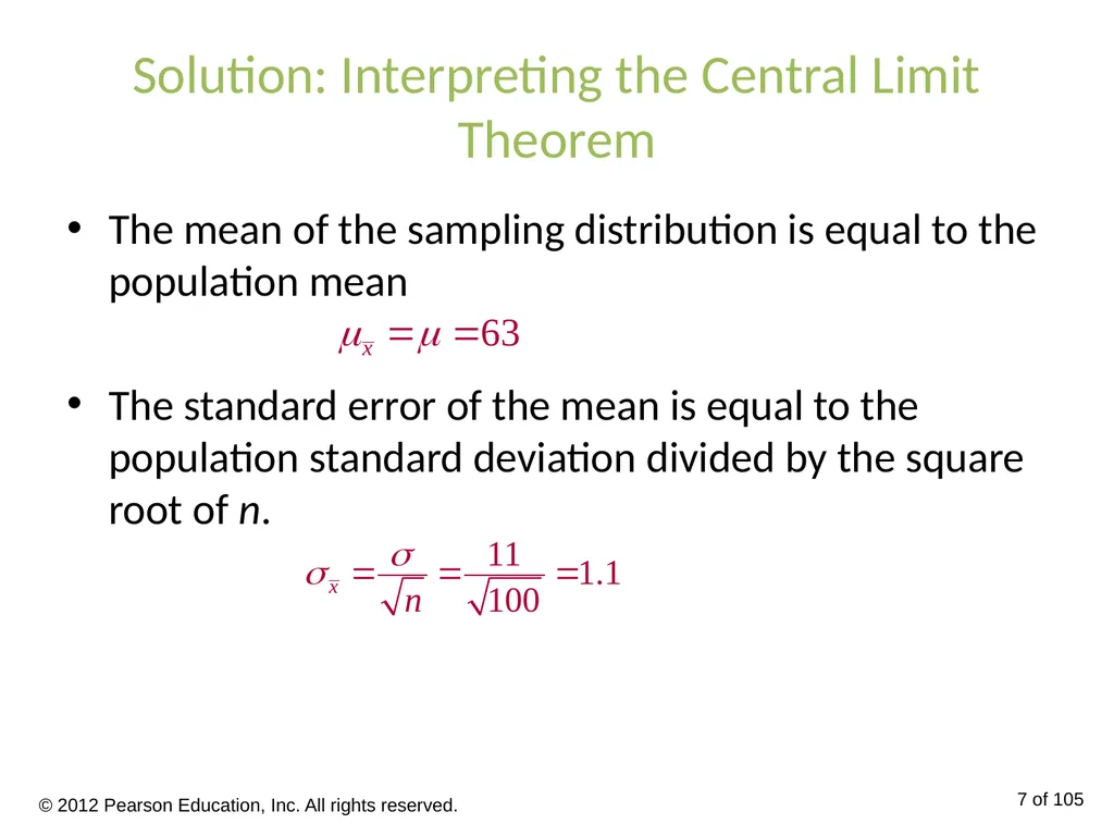
slide7. Solution: Interpreting the Central Limit Theorem The mean of the sampling distribution is equal to the population mean
The standard error of the mean is equal to the population standard deviation divided by the square root of n. © 2012 Pearson Education, Inc. All rights reserved. 7 of 105<br>
slide8. Solution: Interpreting the Central Limit Theorem Since the sample size is greater than 30, the sampling distribution can be approximated by a normal distribution with © 2012 Pearson Education, Inc. All rights reserved. 8 of 105<br>
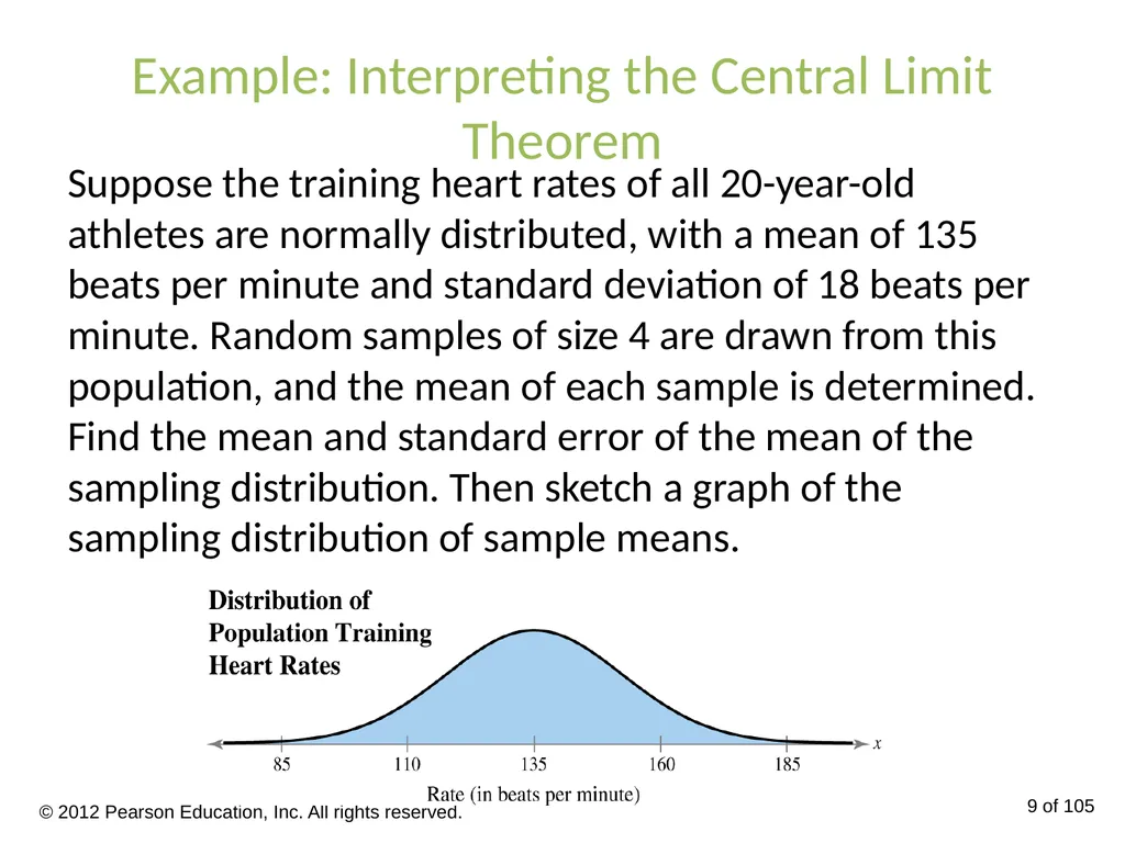
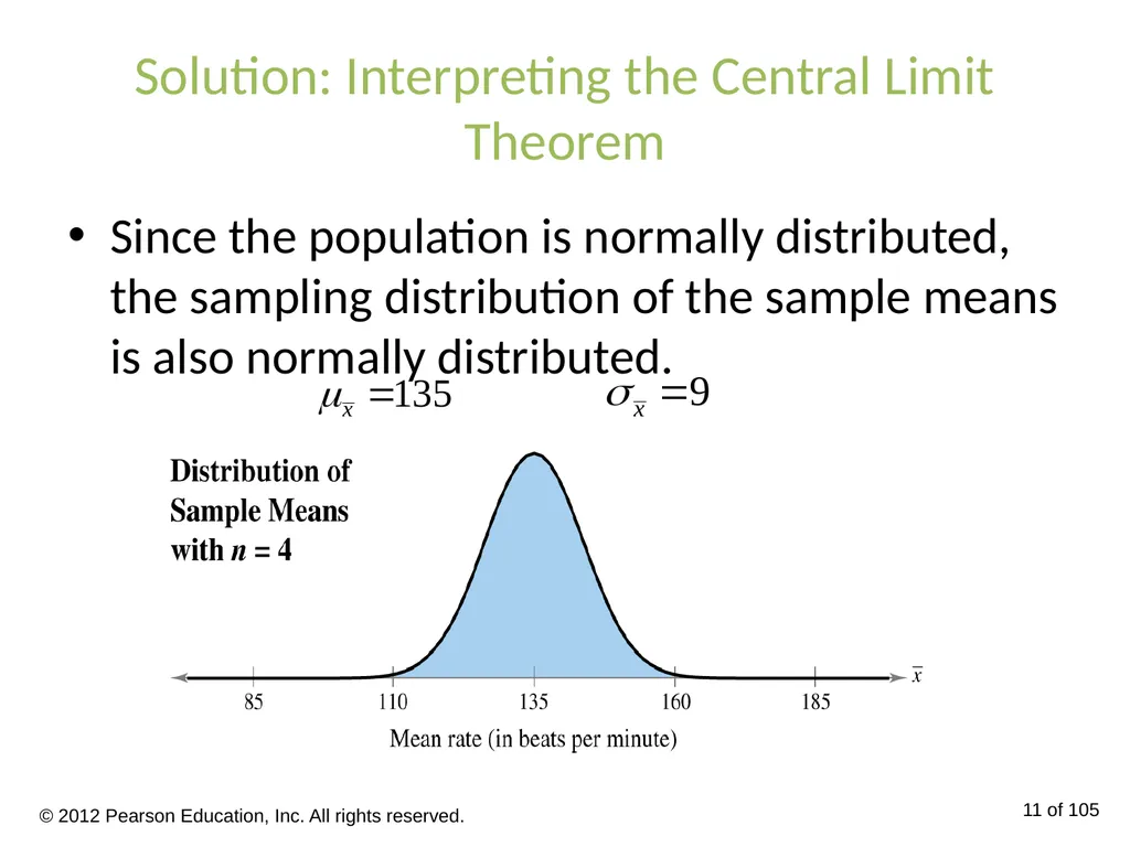
slide9. Example: Interpreting the Central Limit Theorem Suppose the training heart rates of all 20-year-old athletes are normally distributed, with a mean of 135 beats per minute and standard deviation of 18 beats per minute. Random samples of size 4 are drawn from this population, and the mean of each sample is determined. Find the mean and standard error of the mean of the sampling distribution. Then sketch a graph of the sampling distribution of sample means. © 2012 Pearson Education, Inc. All rights reserved. 9 of 105<br>
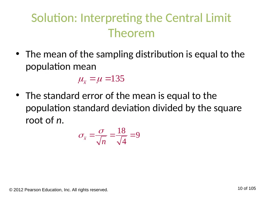
slide10. Solution: Interpreting the Central Limit Theorem The mean of the sampling distribution is equal to the population mean
The standard error of the mean is equal to the population standard deviation divided by the square root of n. © 2012 Pearson Education, Inc. All rights reserved. 10 of 105<br>
slide11. Solution: Interpreting the Central Limit Theorem Since the population is normally distributed, the sampling distribution of the sample means is also normally distributed. © 2012 Pearson Education, Inc. All rights reserved. 11 of 105<br>
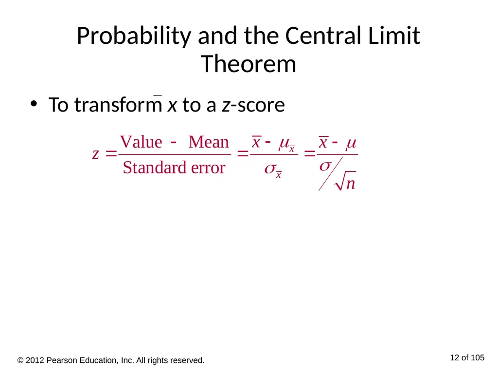
slide12. Probability and the Central Limit Theorem To transform x to a z-score © 2012 Pearson Education, Inc. All rights reserved. 12 of 105<br>
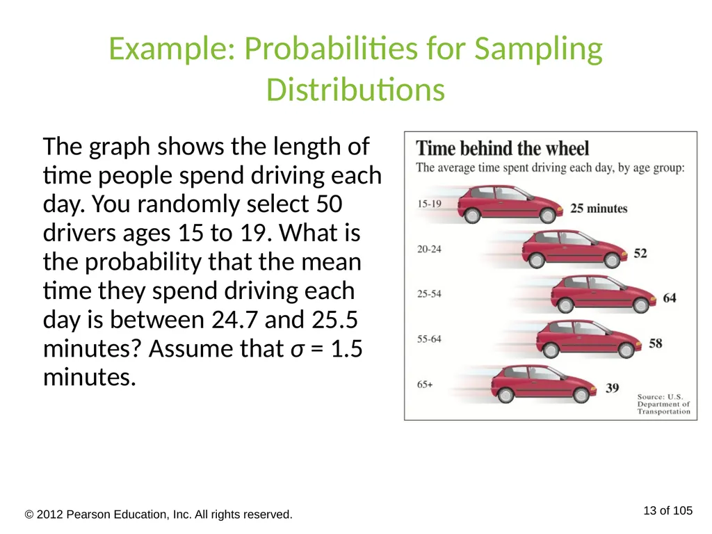
slide13. Example: Probabilities for Sampling Distributions The graph shows the length of time people spend driving each day. You randomly select 50 drivers ages 15 to 19. What is the probability that the mean time they spend driving each day is between 24.7 and 25.5 minutes? Assume that σ = 1.5 minutes. © 2012 Pearson Education, Inc. All rights reserved. 13 of 105<br>
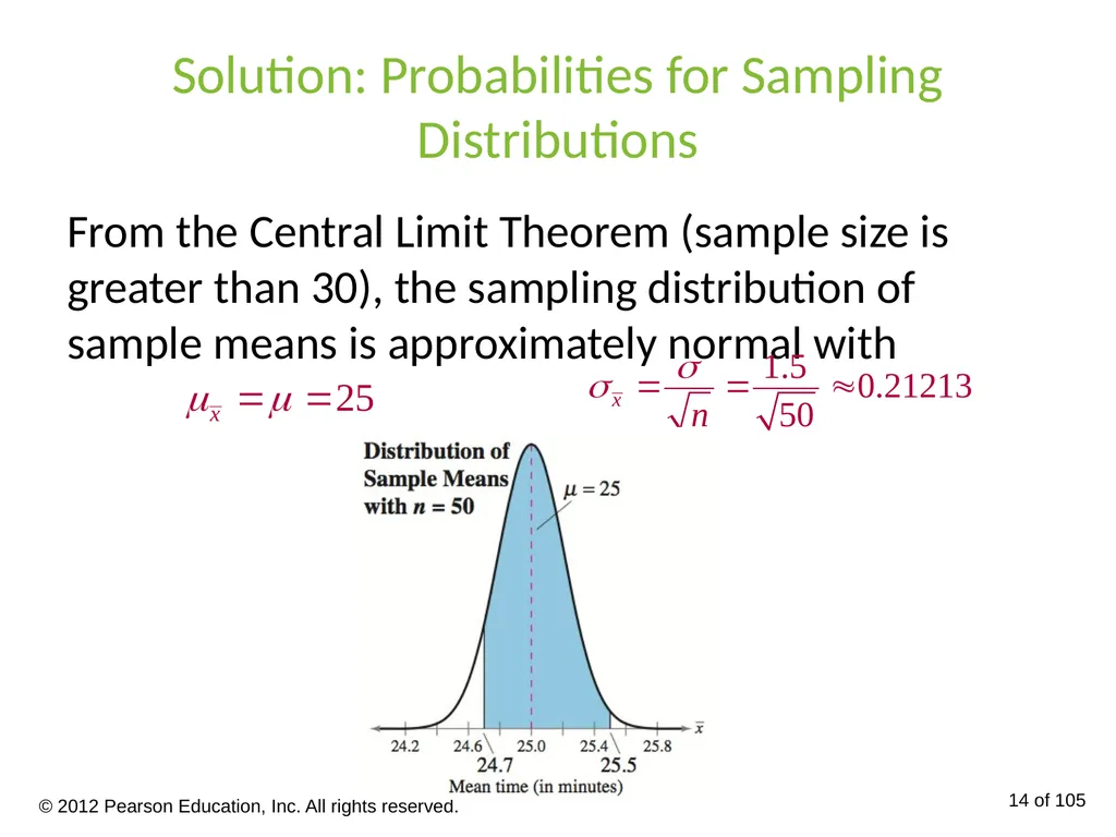
slide14. Solution: Probabilities for Sampling Distributions From the Central Limit Theorem (sample size is greater than 30), the sampling distribution of sample means is approximately normal with © 2012 Pearson Education, Inc. All rights reserved. 14 of 105<br>
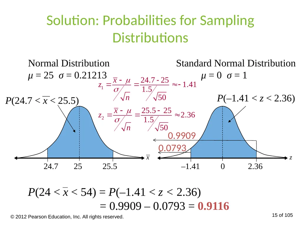
slide15. Solution: Probabilities for Sampling Distributions Normal Distribution μ = 25 σ = 0.21213 25.5 © 2012 Pearson Education, Inc. All rights reserved. 15 of 105<br>
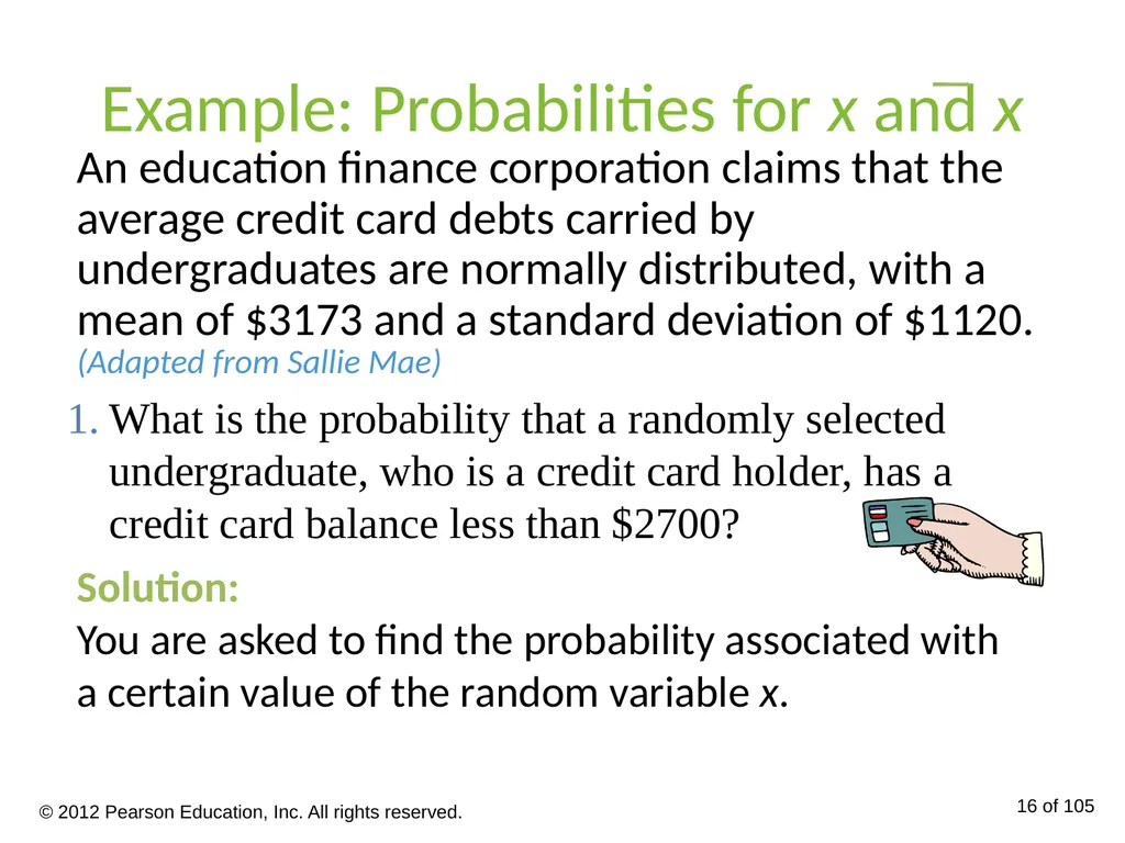
slide16. Example: Probabilities for x and x An education finance corporation claims that the average credit card debts carried by undergraduates are normally distributed, with a mean of $3173 and a standard deviation of $1120. (Adapted from Sallie Mae) Solution:
You are asked to find the probability associated with a certain value of the random variable x. What is the probability that a randomly selected undergraduate, who is a credit card holder, has a credit card balance less than $2700? © 2012 Pearson Education, Inc. All rights reserved. 16 of 105<br>
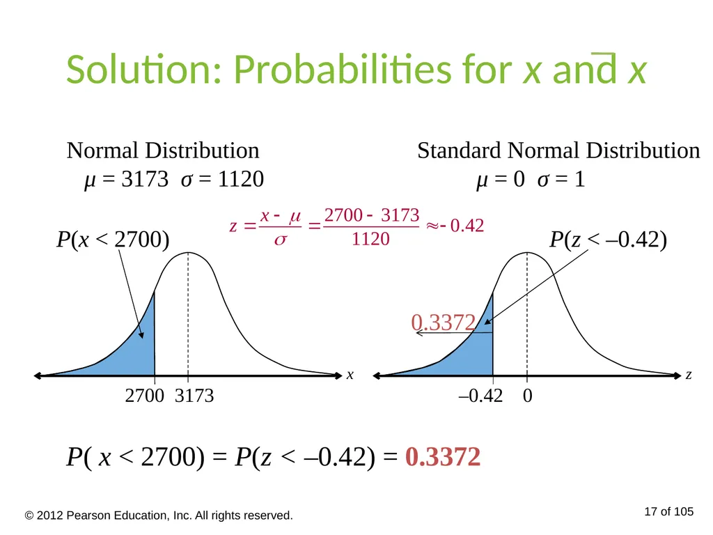
slide17. Solution: Probabilities for x and x P( x < 2700) = P(z < –0.42) = 0.3372 Normal Distribution μ = 3173 σ = 1120 © 2012 Pearson Education, Inc. All rights reserved. 17 of 105<br>
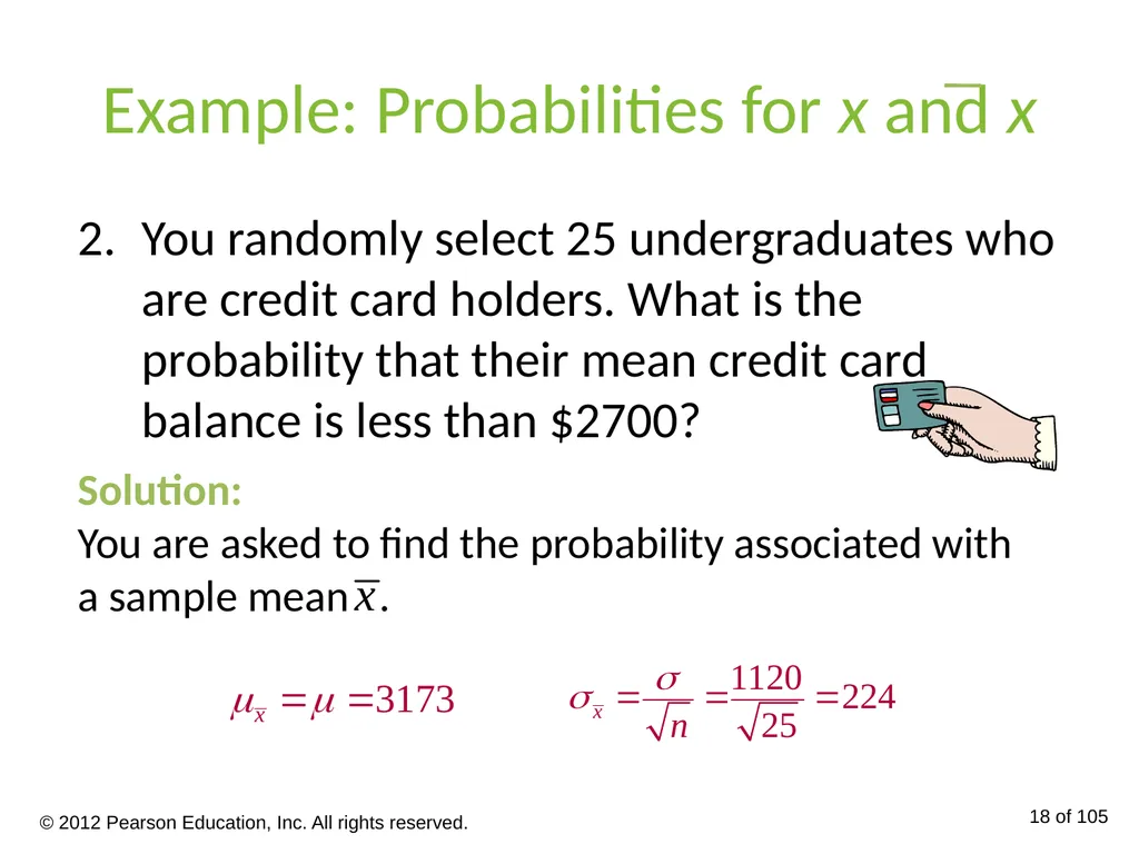
slide18. Example: Probabilities for x and x You randomly select 25 undergraduates who are credit card holders. What is the probability that their mean credit card balance is less than $2700? Solution:
You are asked to find the probability associated with a sample mean . © 2012 Pearson Education, Inc. All rights reserved. 18 of 105<br>
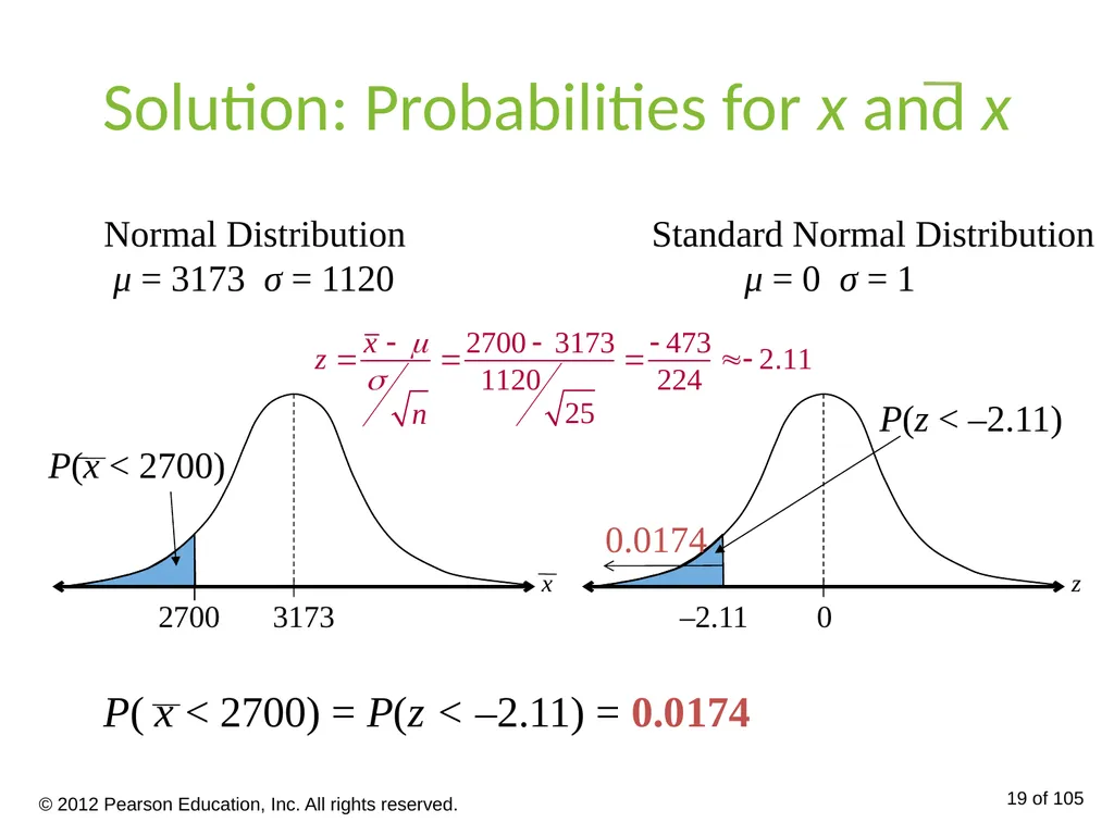
slide19. Solution: Probabilities for x and x Normal Distribution μ = 3173 σ = 1120 © 2012 Pearson Education, Inc. All rights reserved. 19 of 105<br>
slide20. Solution: Probabilities for x and x There is about a 34% chance that an undergraduate will have a balance less than $2700.
There is only about a 2% chance that the mean of a sample of 25 will have a balance less than $2700 (unusual event).
It is possible that the sample is unusual or it is possible that the corporation’s claim that the mean is $3173 is incorrect. © 2012 Pearson Education, Inc. All rights reserved. 20 of 105<br>
slide2. The Central Limit Theorem If samples of size n ≥ 30 are drawn from any population with mean = µ and standard deviation = σ, then the sampling distribution of sample means approximates a normal distribution. The greater the sample size, the better the approximation. © 2012 Pearson Education, Inc. All rights reserved. 2 of 105<br>
slide3. The Central Limit Theorem If the population itself is normally distributed, then the sampling distribution of sample means is normally distribution for any sample size n. © 2012 Pearson Education, Inc. All rights reserved. 3 of 105<br>
slide4. The Central Limit Theorem In either case, the sampling distribution of sample means has a mean equal to the population mean.
The sampling distribution of sample means has a variance equal to 1/n times the variance of the population and a standard deviation equal to the population standard deviation divided by the square root of n. Variance Standard deviation (standard error of the mean) © 2012 Pearson Education, Inc. All rights reserved. 4 of 105 Mean<br>
slide5. The Central Limit Theorem Any Population Distribution Normal Population Distribution Distribution of Sample Means, n ≥ 30 Distribution of Sample Means, (any n) © 2012 Pearson Education, Inc. All rights reserved. 5 of 105<br>
slide6. Example: Interpreting the Central Limit Theorem Cellular phone bills for residents of a city have a mean of $63 and a standard deviation of $11. Random samples of 100 cellular phone bills are drawn from this population and the mean of each sample is determined. Find the mean and standard error of the mean of the sampling distribution. Then sketch a graph of the sampling distribution of sample means. © 2012 Pearson Education, Inc. All rights reserved. 6 of 105<br>
slide7. Solution: Interpreting the Central Limit Theorem The mean of the sampling distribution is equal to the population mean
The standard error of the mean is equal to the population standard deviation divided by the square root of n. © 2012 Pearson Education, Inc. All rights reserved. 7 of 105<br>
slide8. Solution: Interpreting the Central Limit Theorem Since the sample size is greater than 30, the sampling distribution can be approximated by a normal distribution with © 2012 Pearson Education, Inc. All rights reserved. 8 of 105<br>
slide9. Example: Interpreting the Central Limit Theorem Suppose the training heart rates of all 20-year-old athletes are normally distributed, with a mean of 135 beats per minute and standard deviation of 18 beats per minute. Random samples of size 4 are drawn from this population, and the mean of each sample is determined. Find the mean and standard error of the mean of the sampling distribution. Then sketch a graph of the sampling distribution of sample means. © 2012 Pearson Education, Inc. All rights reserved. 9 of 105<br>
slide10. Solution: Interpreting the Central Limit Theorem The mean of the sampling distribution is equal to the population mean
The standard error of the mean is equal to the population standard deviation divided by the square root of n. © 2012 Pearson Education, Inc. All rights reserved. 10 of 105<br>
slide11. Solution: Interpreting the Central Limit Theorem Since the population is normally distributed, the sampling distribution of the sample means is also normally distributed. © 2012 Pearson Education, Inc. All rights reserved. 11 of 105<br>
slide12. Probability and the Central Limit Theorem To transform x to a z-score © 2012 Pearson Education, Inc. All rights reserved. 12 of 105<br>
slide13. Example: Probabilities for Sampling Distributions The graph shows the length of time people spend driving each day. You randomly select 50 drivers ages 15 to 19. What is the probability that the mean time they spend driving each day is between 24.7 and 25.5 minutes? Assume that σ = 1.5 minutes. © 2012 Pearson Education, Inc. All rights reserved. 13 of 105<br>
slide14. Solution: Probabilities for Sampling Distributions From the Central Limit Theorem (sample size is greater than 30), the sampling distribution of sample means is approximately normal with © 2012 Pearson Education, Inc. All rights reserved. 14 of 105<br>
slide15. Solution: Probabilities for Sampling Distributions Normal Distribution μ = 25 σ = 0.21213 25.5 © 2012 Pearson Education, Inc. All rights reserved. 15 of 105<br>
slide16. Example: Probabilities for x and x An education finance corporation claims that the average credit card debts carried by undergraduates are normally distributed, with a mean of $3173 and a standard deviation of $1120. (Adapted from Sallie Mae) Solution:
You are asked to find the probability associated with a certain value of the random variable x. What is the probability that a randomly selected undergraduate, who is a credit card holder, has a credit card balance less than $2700? © 2012 Pearson Education, Inc. All rights reserved. 16 of 105<br>
slide17. Solution: Probabilities for x and x P( x < 2700) = P(z < –0.42) = 0.3372 Normal Distribution μ = 3173 σ = 1120 © 2012 Pearson Education, Inc. All rights reserved. 17 of 105<br>
slide18. Example: Probabilities for x and x You randomly select 25 undergraduates who are credit card holders. What is the probability that their mean credit card balance is less than $2700? Solution:
You are asked to find the probability associated with a sample mean . © 2012 Pearson Education, Inc. All rights reserved. 18 of 105<br>
slide19. Solution: Probabilities for x and x Normal Distribution μ = 3173 σ = 1120 © 2012 Pearson Education, Inc. All rights reserved. 19 of 105<br>
slide20. Solution: Probabilities for x and x There is about a 34% chance that an undergraduate will have a balance less than $2700.
There is only about a 2% chance that the mean of a sample of 25 will have a balance less than $2700 (unusual event).
It is possible that the sample is unusual or it is possible that the corporation’s claim that the mean is $3173 is incorrect. © 2012 Pearson Education, Inc. All rights reserved. 20 of 105<br>