
Monetary Regimes For Emerging Markets Panel on
LS
Published · 39 slides · 0 views
1 / 1


Description
Monetary Regimes For Emerging Markets Panel on Monetary Policy, Conference on Monetary Policy and Financial Stability in Emerging Markets, NBER Central Bank of the Republic of Turkey, Istanbul, Turkey, June 13-14, 2014 Jeffrey Frankel
Related Topics
Share
Embed code
Download this presentation From Below
"Monetary Regimes For Emerging Markets Panel on" is the property of its rightful owner. Permission is granted to download and print the materials on this website for personal, non-commercial use only, and to display it on your personal computer provided you do not modify the materials and that you retain all copyright notices contained in the materials. By downloading content from our website, you accept the terms of this agreement.
Presentation Transcript
01
Monetary Regimes
For Emerging Markets Panel on Monetary Policy,
Conference on Monetary Policy
and Financial Stability in Emerging Markets,
NBER & Central Bank of the Republic of Turkey,
Istanbul, Turkey, June 13-14, 2014 Jeffrey Frankel
Harvard University & NBER<br>
Harvard University & NBER<br>
02
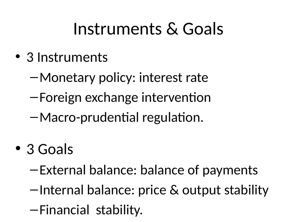
Instruments & Goals 3 Instruments
Monetary policy: interest rate
Foreign exchange intervention
Macro-prudential regulation.
3 Goals
External balance: balance of payments
Internal balance: price & output stability
Financial stability.<br>
Monetary policy: interest rate
Foreign exchange intervention
Macro-prudential regulation.
3 Goals
External balance: balance of payments
Internal balance: price & output stability
Financial stability.<br>
03
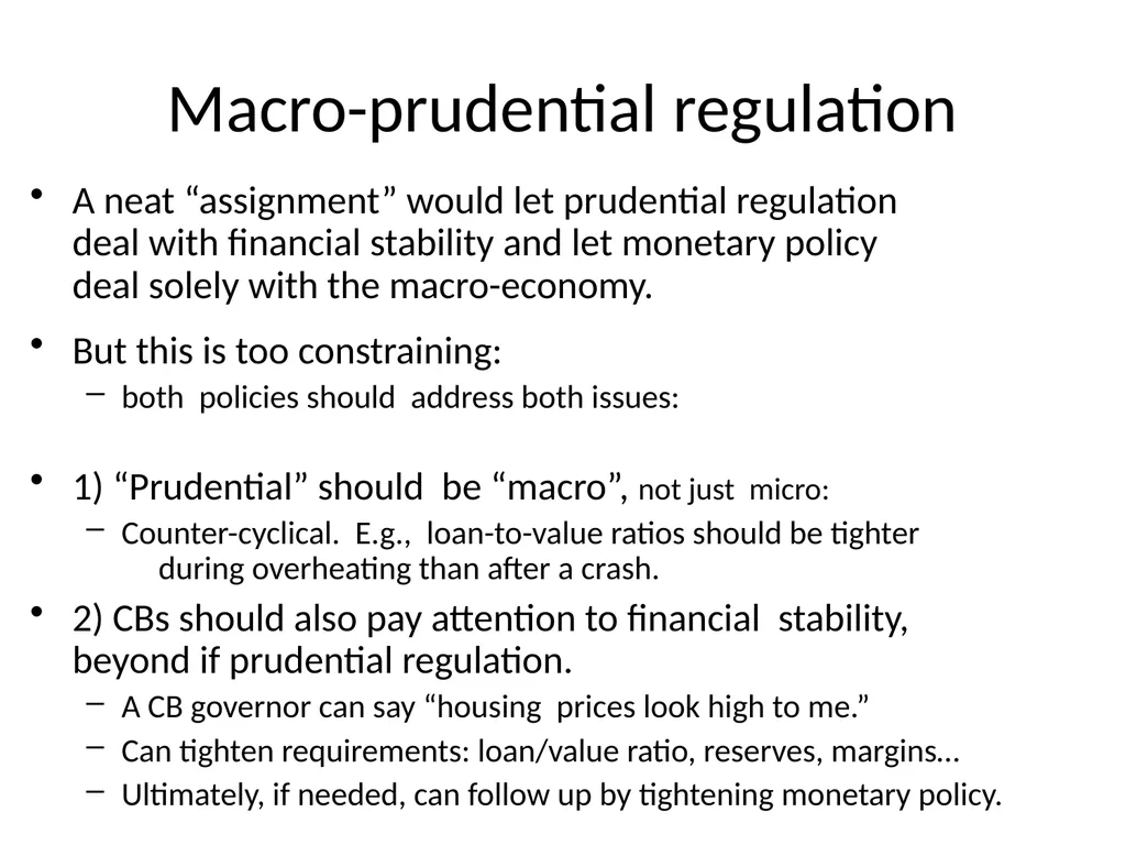
Macro-prudential regulation A neat “assignment” would let prudential regulation
deal with financial stability and let monetary policy
deal solely with the macro-economy.
But this is too constraining:
both policies should address both issues:
1) “Prudential” should be “macro”, not just micro:
Counter-cyclical. E.g., loan-to-value ratios should be tighter during overheating than after a crash.
2) CBs should also pay attention to financial stability, beyond if prudential regulation.
A CB governor can say “housing prices look high to me.”
Can tighten requirements: loan/value ratio, reserves, margins…
Ultimately, if needed, can follow up by tightening monetary policy.<br>
But this is too constraining:
both policies should address both issues:
1) “Prudential” should be “macro”, not just micro:
Counter-cyclical. E.g., loan-to-value ratios should be tighter during overheating than after a crash.
2) CBs should also pay attention to financial stability, beyond if prudential regulation.
A CB governor can say “housing prices look high to me.”
Can tighten requirements: loan/value ratio, reserves, margins…
Ultimately, if needed, can follow up by tightening monetary policy.<br>
04
The Choice of Monetary Regimes
for Emerging Markets How are EMs structurally different
from Advanced Economies?
Choice of exchange rate regime
Alternative anchors for monetary policy<br>
Choice of exchange rate regime
Alternative anchors for monetary policy<br>
05
I. How are EMs different
from Advanced Economies? Monetary policy-maker has more need for credibility
a) due to high-inflation histories,
b) absence of credible institutions,
c) or political pressure to monetize big budget deficits.
Economy is more exposed to supply shocks
a) such as natural disasters,
b) other weather events,
c) strikes and social unrest,
d) productivity shocks.
More exposed to terms of trade shocks
because country tends to be price-taker
Volatility in price of export commodity on world markets
Volatility in price of imports like oil on world markets.<br>
a) due to high-inflation histories,
b) absence of credible institutions,
c) or political pressure to monetize big budget deficits.
Economy is more exposed to supply shocks
a) such as natural disasters,
b) other weather events,
c) strikes and social unrest,
d) productivity shocks.
More exposed to terms of trade shocks
because country tends to be price-taker
Volatility in price of export commodity on world markets
Volatility in price of imports like oil on world markets.<br>
06
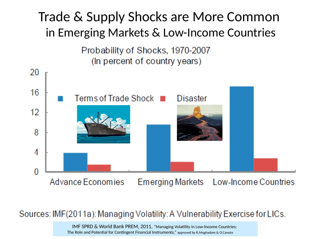
Trade & Supply Shocks are More Common
in Emerging Markets & Low-Income Countries IMF SPRD & World Bank PREM, 2011, “Managing Volatility in Low-Income Countries:
The Role and Potential for Contingent Financial Instruments,” approved by R.Moghadam & O.Canuto<br>
07
II. What is the desirable exchange rate regime? Very small, very open, economies will continue to want to fix their exchange rates, in most cases.
Most countries are in between,
particularly middle-sized middle-income countries.
Most of these countries should have intermediate exchange rate regimes,
neither firm fixing nor free floating.
They include band & basket arrangements.<br>
Most countries are in between,
particularly middle-sized middle-income countries.
Most of these countries should have intermediate exchange rate regimes,
neither firm fixing nor free floating.
They include band & basket arrangements.<br>
08
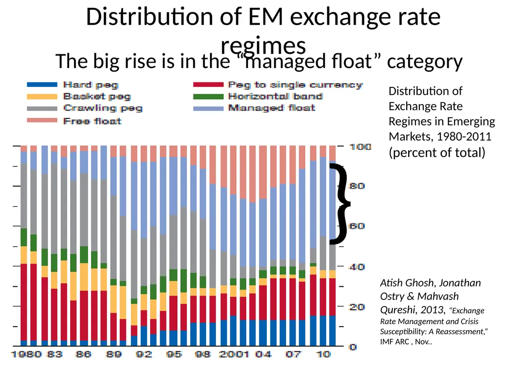
Distribution of EM exchange rate regimes Atish Ghosh, Jonathan Ostry & Mahvash Qureshi, 2013, “Exchange Rate Management and Crisis Susceptibility: A Reassessment,”
IMF ARC , Nov.. The big rise is in the “managed float” category } Distribution of Exchange Rate Regimes in Emerging Markets, 1980-2011
(percent of total)<br>
(percent of total)<br>
09
So I reject the Corners Hypothesis. But Stan Fischer has a good point: giving speculators
a target to shoot at is often a losing proposition (“disastrous”),
such as the boundary of a declared band.
A particular intermediate regime could be useful, a systematic sort of managed floating:
A rule could say that for every 1% of Exchange Market Pressure, the central bank takes x % as an appreciation of the currency and (1-x) % as an increase in reserves (relative to the monetary base).
This arrangement, tho rather obvious, has seldom been formalized.
The parameter x calibrates exchange rate flexibility,
and can range from 0 (fixing) to close to 1 (full flexibility).
Thus one can have ½ monetary independence + ½ exchange rate stability.<br>
such as the boundary of a declared band.
A particular intermediate regime could be useful, a systematic sort of managed floating:
A rule could say that for every 1% of Exchange Market Pressure, the central bank takes x % as an appreciation of the currency and (1-x) % as an increase in reserves (relative to the monetary base).
This arrangement, tho rather obvious, has seldom been formalized.
The parameter x calibrates exchange rate flexibility,
and can range from 0 (fixing) to close to 1 (full flexibility).
Thus one can have ½ monetary independence + ½ exchange rate stability.<br>
10
refutes the corners hypothesis,
but without capital controls,
without violating the Impossible Trinity,
and even without giving speculators a line to shoot at.
≈ what some central banks do anyway.
Attempts at econometric estimation
G.Adler & C.Tovar, 2011, “Foreign Exchange Intervention: A Shield Against Appreciation Winds?” IMF WP 11/165.
J.Frankel & D, Xie, 2010, “Estimation of De Facto Flexibility Parameter and Basket Weights in Evolving Exchange Rate Regimes,” AER. Systematic managed floating<br>
but without capital controls,
without violating the Impossible Trinity,
and even without giving speculators a line to shoot at.
≈ what some central banks do anyway.
Attempts at econometric estimation
G.Adler & C.Tovar, 2011, “Foreign Exchange Intervention: A Shield Against Appreciation Winds?” IMF WP 11/165.
J.Frankel & D, Xie, 2010, “Estimation of De Facto Flexibility Parameter and Basket Weights in Evolving Exchange Rate Regimes,” AER. Systematic managed floating<br>
11
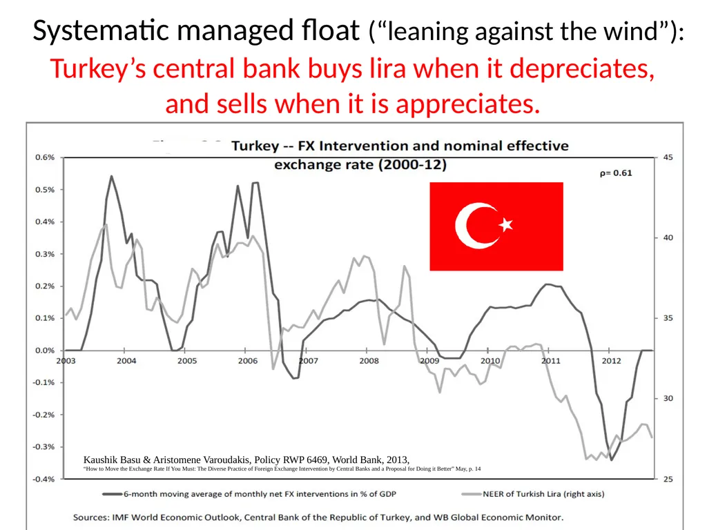
Systematic managed float (“leaning against the wind”): Kaushik Basu & Aristomene Varoudakis, Policy RWP 6469, World Bank, 2013,
“How to Move the Exchange Rate If You Must: The Diverse Practice of Foreign Exchange Intervention by Central Banks and a Proposal for Doing it Better” May, p. 14 Turkey’s central bank buys lira when it depreciates,
and sells when it is appreciates.<br>
12
Korea & Singapore took them mostly in the form of reserves, GS Global ECS Research less-managed floating more-managed floating Example: Renewed capital inflows to Asia in 2010 while India & Malaysia took them mostly
in the form of currency appreciation. Slope
= 1/x<br>
13
Renewed inflows in 2010 in Latin America less-managed floating more-managed floating but as appreciation in Chile & Colombia. were reflected mostly as reserve accumulation in Peru, Source: GS Global ECS Research Slope
= 1/x<br>
14
III: If the exchange rate is not to be
the anchor for monetary policy, what is? The need for an alternative anchor led many EMs to IT,
after the currency crises of the late 1990s pushed them off exchange rate targets.
IT (Inflation Targeting) was in many ways successful.
Two problems with IT:
Neglect of asset bubbles
Neglect of exogenous supply & trade shocks.
Remember the textbook maxim: the exchange rate should accommodate terms of trade shocks.
If IT sets the CPI, it doesn’t allow the exchange rate to rise & fall with the terms of trade.
When the world price of imported oil rises, a literal CPI target says to tighten monetary policy enough to appreciate the currency,
the opposite of accommodating the adverse trade shock.<br>
after the currency crises of the late 1990s pushed them off exchange rate targets.
IT (Inflation Targeting) was in many ways successful.
Two problems with IT:
Neglect of asset bubbles
Neglect of exogenous supply & trade shocks.
Remember the textbook maxim: the exchange rate should accommodate terms of trade shocks.
If IT sets the CPI, it doesn’t allow the exchange rate to rise & fall with the terms of trade.
When the world price of imported oil rises, a literal CPI target says to tighten monetary policy enough to appreciate the currency,
the opposite of accommodating the adverse trade shock.<br>
15
Nominal GDP Targeting NGDPT is more robust with respect to
supply shocks & terms of trade shocks,
compared to the alternative of IT.
The logic holds whether the immediate aim is
Disinflation (as in 1980s, and today among some EMs);
Monetary stimulus (as among big ACs recently);
or just staying the course.<br>
compared to the alternative of IT.
The logic holds whether the immediate aim is
Disinflation (as in 1980s, and today among some EMs);
Monetary stimulus (as among big ACs recently);
or just staying the course.<br>
16
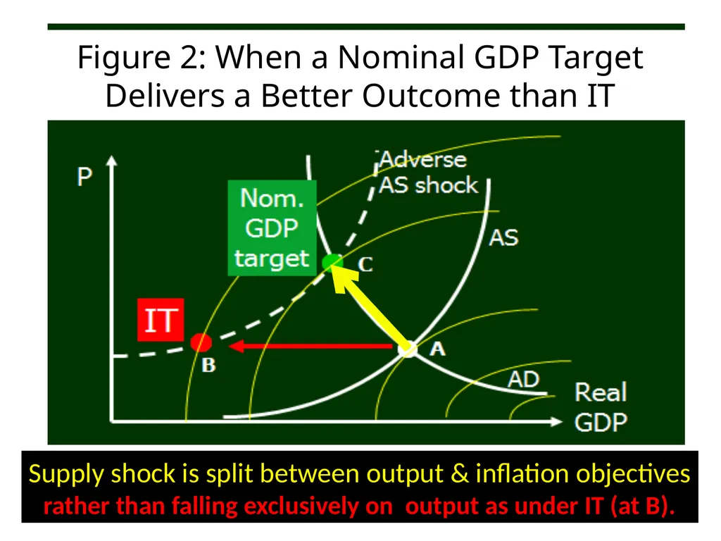
Figure 2: When a Nominal GDP Target
Delivers a Better Outcome than IT Supply shock is split between output & inflation objectives
rather than falling exclusively on output as under IT (at B).<br>
rather than falling exclusively on output as under IT (at B).<br>
17
Last point: NGDPT for EMs The proponents of Nominal GDP Targets
have focused on the biggest countries.
But middle-size, middle-income countries are better candidates.
Why? They suffer bigger supply shocks & trade shocks.
Evidence suggests that the AS curve is indeed sufficiently steep so that NGDPT minimizes quadratic loss function:
“Nominal GDP Targeting for Middle-Income Countries,” June 2014 for Central Bank Review, of CBRT.
Conclusion: EMs should consider NGDPT as a serious alternative to IT & exchange rate targeting.<br>
But middle-size, middle-income countries are better candidates.
Why? They suffer bigger supply shocks & trade shocks.
Evidence suggests that the AS curve is indeed sufficiently steep so that NGDPT minimizes quadratic loss function:
“Nominal GDP Targeting for Middle-Income Countries,” June 2014 for Central Bank Review, of CBRT.
Conclusion: EMs should consider NGDPT as a serious alternative to IT & exchange rate targeting.<br>
18
Appendices Boom-bust cycle in EM capital flows
External shocks
“Risk off”
US interest rates
Which countries withstand shocks
In 2008-09 and previous crises?
In 2013 temper tantrum?<br>
External shocks
“Risk off”
US interest rates
Which countries withstand shocks
In 2008-09 and previous crises?
In 2013 temper tantrum?<br>
19
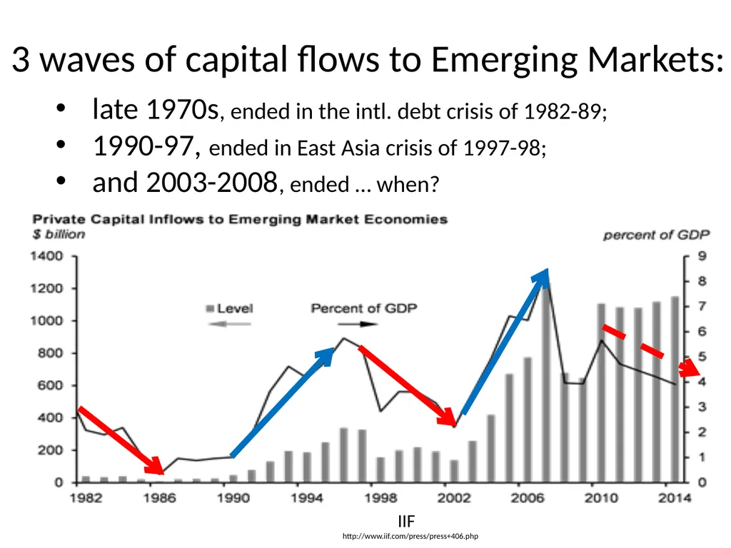
3 waves of capital flows to Emerging Markets: IIF
http://www.iif.com/press/press+406.php late 1970s, ended in the intl. debt crisis of 1982-89;
1990-97, ended in East Asia crisis of 1997-98;
and 2003-2008, ended … when?<br>
1990-97, ended in East Asia crisis of 1997-98;
and 2003-2008, ended … when?<br>
20
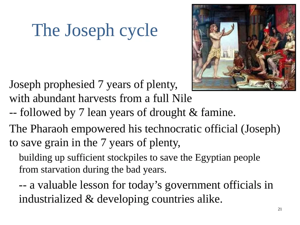
The Joseph cycle Joseph prophesied 7 years of plenty,
with abundant harvests from a full Nile
-- followed by 7 lean years of drought & famine.
The Pharaoh empowered his technocratic official (Joseph) to save grain in the 7 years of plenty,
building up sufficient stockpiles to save the Egyptian people from starvation during the bad years.
-- a valuable lesson for today’s government officials in industrialized & developing countries alike. 21<br>
The Pharaoh empowered his technocratic official (Joseph) to save grain in the 7 years of plenty,
building up sufficient stockpiles to save the Egyptian people from starvation during the bad years.
-- a valuable lesson for today’s government officials in industrialized & developing countries alike. 21<br>
21
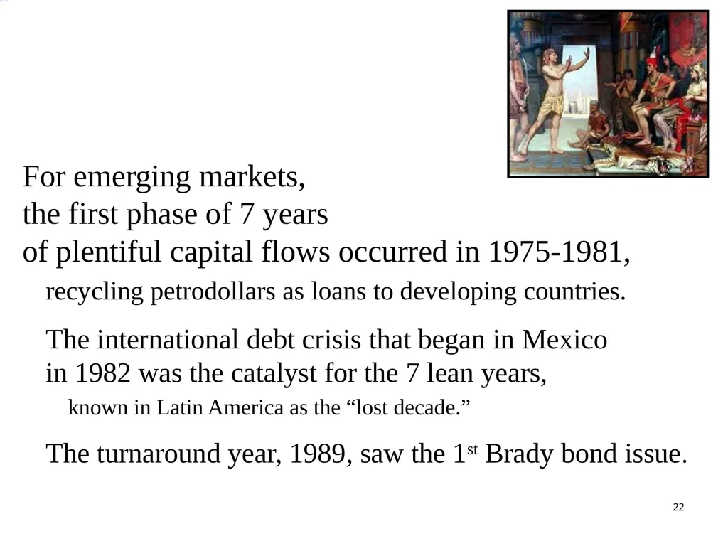
Biblical cycle, cont. For emerging markets,
the first phase of 7 years
of plentiful capital flows occurred in 1975-1981,
recycling petrodollars as loans to developing countries.
The international debt crisis that began in Mexico in 1982 was the catalyst for the 7 lean years,
known in Latin America as the “lost decade.”
The turnaround year, 1989, saw the 1st Brady bond issue. 22<br>
recycling petrodollars as loans to developing countries.
The international debt crisis that began in Mexico in 1982 was the catalyst for the 7 lean years,
known in Latin America as the “lost decade.”
The turnaround year, 1989, saw the 1st Brady bond issue. 22<br>
22
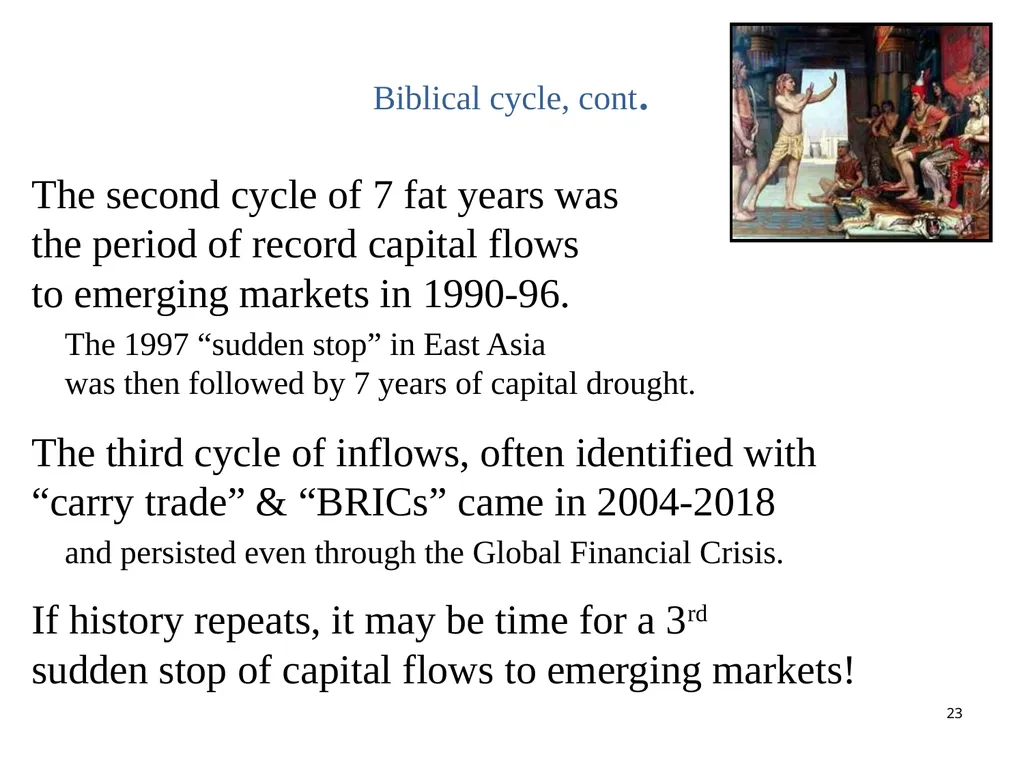
Biblical cycle, cont. The second cycle of 7 fat years was
the period of record capital flows
to emerging markets in 1990-96.
The 1997 “sudden stop” in East Asia was then followed by 7 years of capital drought.
The third cycle of inflows, often identified with “carry trade” & “BRICs” came in 2004-2018
and persisted even through the Global Financial Crisis.
If history repeats, it may be time for a 3rd sudden stop of capital flows to emerging markets! 23<br>
The 1997 “sudden stop” in East Asia was then followed by 7 years of capital drought.
The third cycle of inflows, often identified with “carry trade” & “BRICs” came in 2004-2018
and persisted even through the Global Financial Crisis.
If history repeats, it may be time for a 3rd sudden stop of capital flows to emerging markets! 23<br>
23
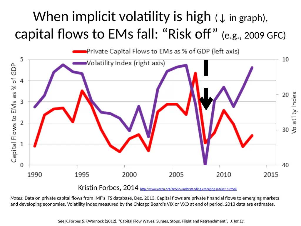
When implicit volatility is high (↓ in graph),
capital flows to EMs fall: “Risk off” (e.g., 2009 GFC) Kristin Forbes, 2014 http://www.voxeu.org/article/understanding-emerging-market-turmoil Notes: Data on private capital flows from IMF's IFS database, Dec. 2013. Capital flows are private financial flows to emerging markets and developing economies. Volatility index measured by the Chicago Board's VIX or VXO at end of period. 2013 data are estimates. See K.Forbes & F.Warnock (2012), “Capital Flow Waves: Surges, Stops, Flight and Retrenchment”, J. Int.Ec.<br>
24
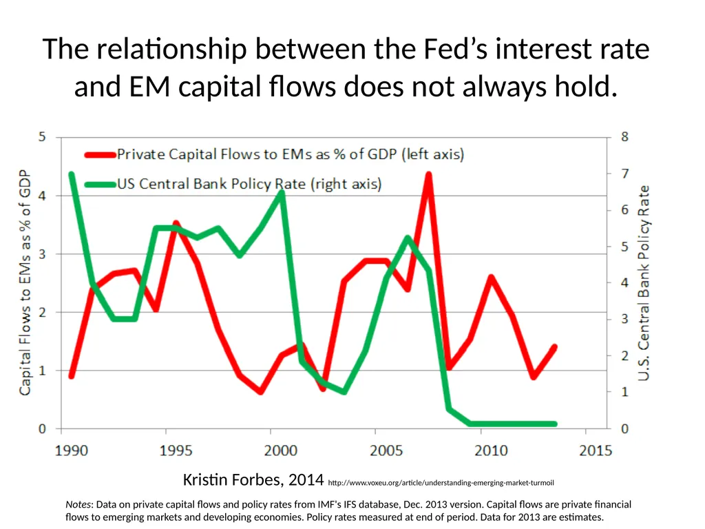
The role of US monetary policy Low US real interest rates contributed to EM flows
in late 1970s, early 1990s, and early 2000s.
The Volcker tightening of 1980-82 precipitated the international debt crisis of 1982.
The Fed tightening of 1994 helped precipitate the Mexican peso crisis of that year.
But the correlation is not always there.<br>
The Volcker tightening of 1980-82 precipitated the international debt crisis of 1982.
The Fed tightening of 1994 helped precipitate the Mexican peso crisis of that year.
But the correlation is not always there.<br>
25
The relationship between the Fed’s interest rate
and EM capital flows does not always hold. Kristin Forbes, 2014 http://www.voxeu.org/article/understanding-emerging-market-turmoil Notes: Data on private capital flows and policy rates from IMF's IFS database, Dec. 2013 version. Capital flows are private financial flows to emerging markets and developing economies. Policy rates measured at end of period. Data for 2013 are estimates.<br>
26
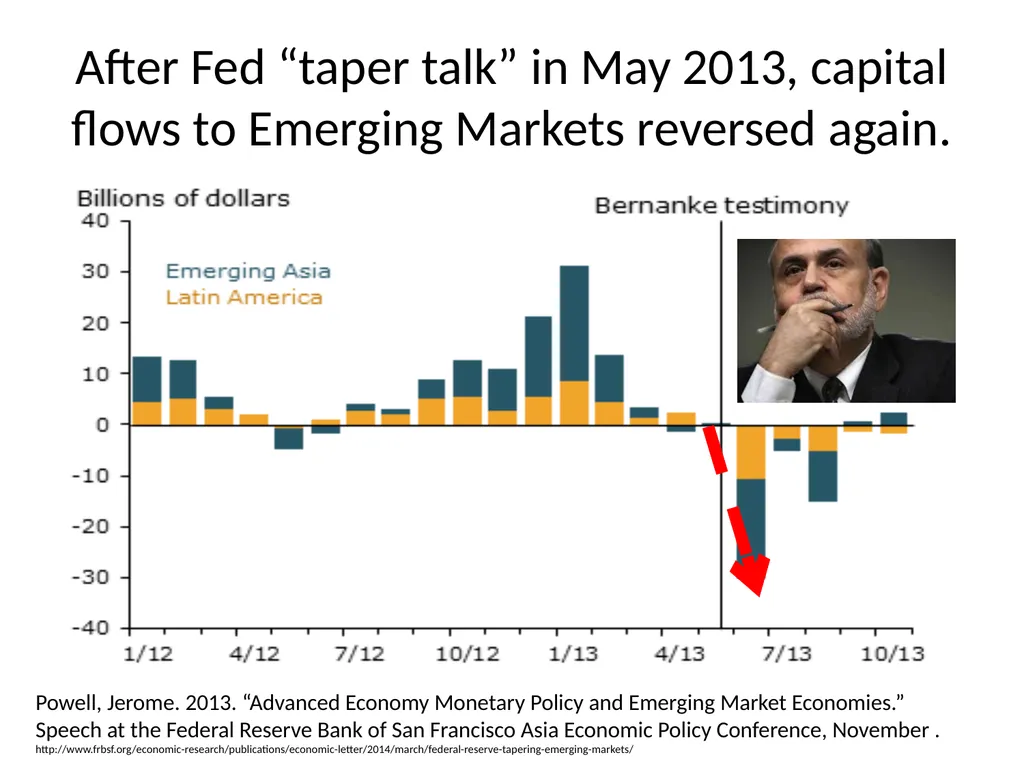
After Fed “taper talk” in May 2013, capital flows to Emerging Markets reversed again. Powell, Jerome. 2013. “Advanced Economy Monetary Policy and Emerging Market Economies.”
Speech at the Federal Reserve Bank of San Francisco Asia Economic Policy Conference, November .
http://www.frbsf.org/economic-research/publications/economic-letter/2014/march/federal-reserve-tapering-emerging-markets/<br>
27
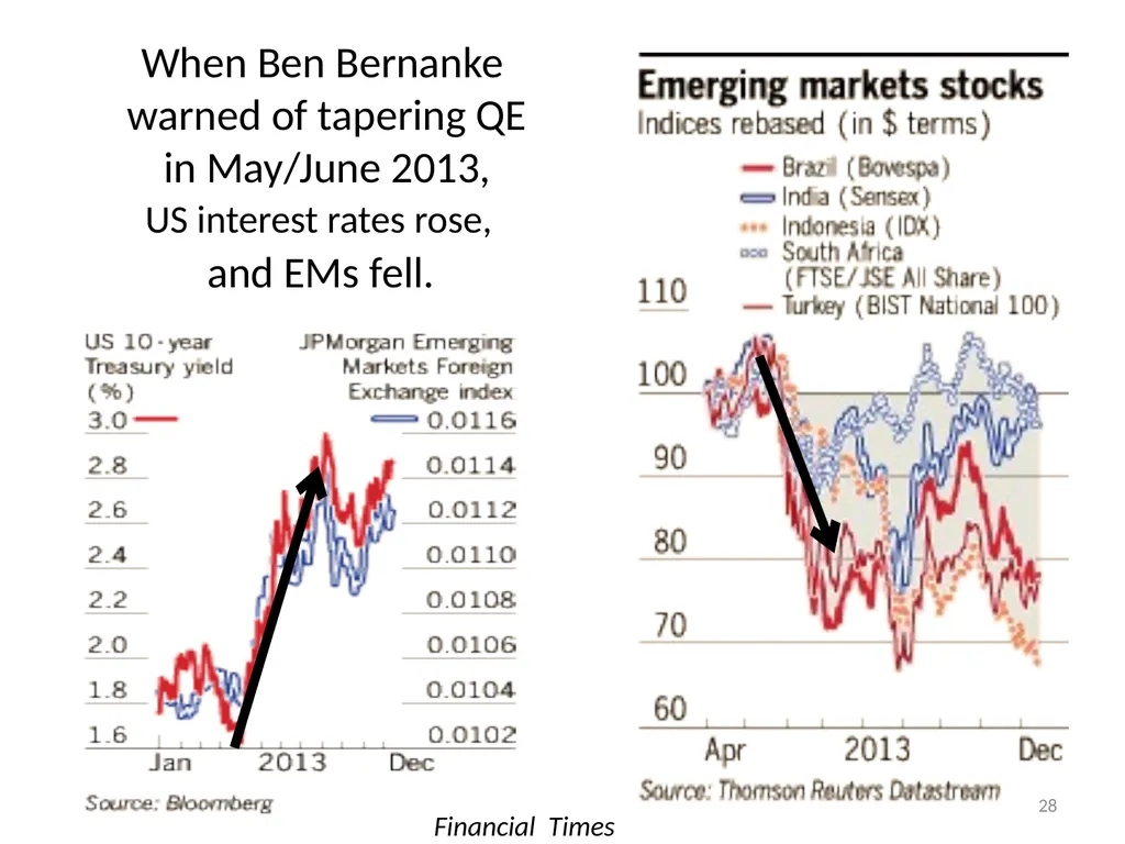
28 When Ben Bernanke
warned of tapering QE
in May/June 2013, Financial Times US interest rates rose, and EMs fell.<br>
in May/June 2013, Financial Times US interest rates rose, and EMs fell.<br>
28
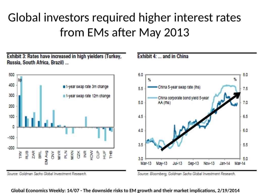
Global investors required higher interest rates from EMs after May 2013 Global Economics Weekly: 14/07 - The downside risks to EM growth and their market implications, 2/19/2014<br>
29
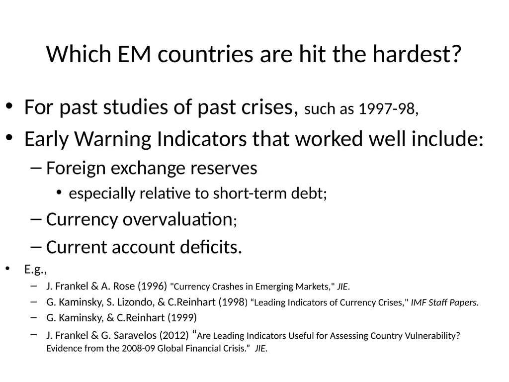
Which EM countries are hit the hardest? For past studies of past crises, such as 1997-98,
Early Warning Indicators that worked well include:
Foreign exchange reserves
especially relative to short-term debt;
Currency overvaluation;
Current account deficits.
E.g.,
J. Frankel & A. Rose (1996) "Currency Crashes in Emerging Markets," JIE.
G. Kaminsky, S. Lizondo, & C.Reinhart (1998) “Leading Indicators of Currency Crises," IMF Staff Papers.
G. Kaminsky, & C.Reinhart (1999)
J. Frankel & G. Saravelos (2012) “Are Leading Indicators Useful for Assessing Country Vulnerability? Evidence from the 2008-09 Global Financial Crisis.” JIE.<br>
Early Warning Indicators that worked well include:
Foreign exchange reserves
especially relative to short-term debt;
Currency overvaluation;
Current account deficits.
E.g.,
J. Frankel & A. Rose (1996) "Currency Crashes in Emerging Markets," JIE.
G. Kaminsky, S. Lizondo, & C.Reinhart (1998) “Leading Indicators of Currency Crises," IMF Staff Papers.
G. Kaminsky, & C.Reinhart (1999)
J. Frankel & G. Saravelos (2012) “Are Leading Indicators Useful for Assessing Country Vulnerability? Evidence from the 2008-09 Global Financial Crisis.” JIE.<br>
30
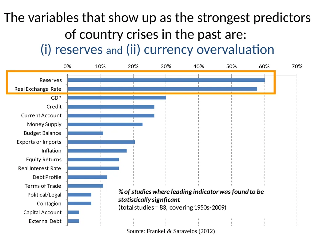
The variables that show up as the strongest predictors of country crises in the past are: Source: Frankel & Saravelos (2012) (i) reserves and (ii) currency overvaluation<br>
31
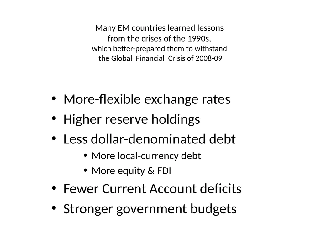
Many EM countries learned lessons
from the crises of the 1990s,
which better-prepared them to withstand
the Global Financial Crisis of 2008-09 More-flexible exchange rates
Higher reserve holdings
Less dollar-denominated debt
More local-currency debt
More equity & FDI
Fewer Current Account deficits
Stronger government budgets<br>
Higher reserve holdings
Less dollar-denominated debt
More local-currency debt
More equity & FDI
Fewer Current Account deficits
Stronger government budgets<br>
32
Foreign exchange reserves are useful One purpose is dampening appreciation,
thus limiting current account deficits.
Another is the precautionary motive.
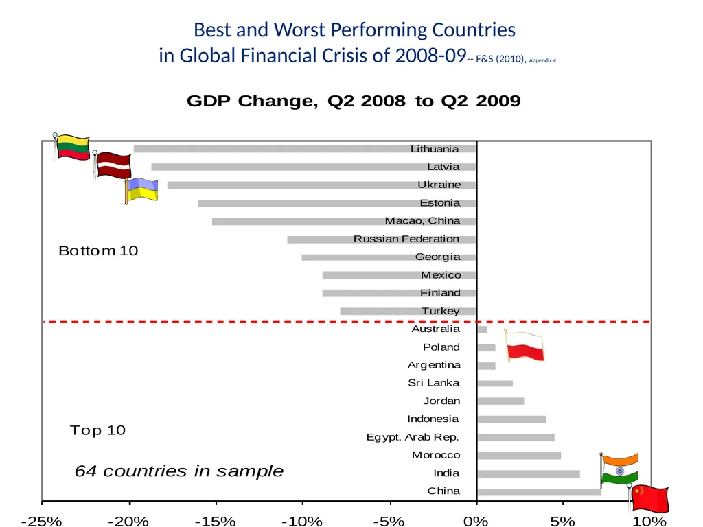
The best predictor of who got hit in the 2008 Global Financial Crisis was reserves
Frankel & Saravelos (2012).
Dominguez & Ito.
This was the same Warning Indicator that also had worked in the most studies of earlier crises.<br>
thus limiting current account deficits.
Another is the precautionary motive.
The best predictor of who got hit in the 2008 Global Financial Crisis was reserves
Frankel & Saravelos (2012).
Dominguez & Ito.
This was the same Warning Indicator that also had worked in the most studies of earlier crises.<br>
33
Best and Worst Performing Countries
in Global Financial Crisis of 2008-09-- F&S (2010), Appendix 4<br>
34
Which EM countries were hit the hardest
by the “taper tantrum” of May-June 2013? Those with big current account deficits,
or with exchange rate overvaluation.
Reserves did not seem to help this time.
E.g.,
B. Eichengreen & P. Gupta (2013) “Tapering Talk: The Impact of Expectations of Reduced Federal Reserve Security Purchases on Emerging Markets,” Working Paper.
Jon Hill (2014), “Exploring Early Warning Indicators for Financial Crises in 2013 & 2014,” HKS, April.<br>
or with exchange rate overvaluation.
Reserves did not seem to help this time.
E.g.,
B. Eichengreen & P. Gupta (2013) “Tapering Talk: The Impact of Expectations of Reduced Federal Reserve Security Purchases on Emerging Markets,” Working Paper.
Jon Hill (2014), “Exploring Early Warning Indicators for Financial Crises in 2013 & 2014,” HKS, April.<br>
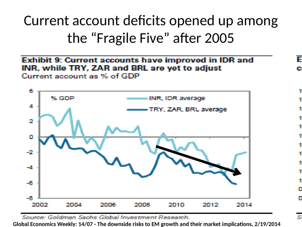
35
Current account deficits opened up among the “Fragile Five” after 2005 Global Economics Weekly: 14/07 - The downside risks to EM growth and their market implications, 2/19/2014<br>
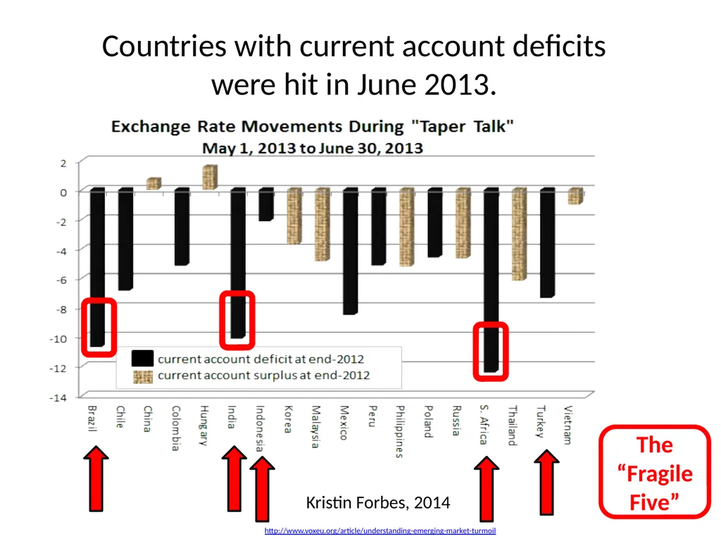
36
Countries with current account deficits
were hit in June 2013. Kristin Forbes, 2014
http://www.voxeu.org/article/understanding-emerging-market-turmoil The “Fragile Five”<br>
37
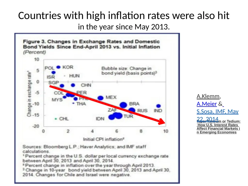
Countries with high inflation rates were also hit
in the year since May 2013. Taper Tantrum or Tedium: How U.S. Interest Rates Affect Financial Markets in Emerging Economies A.Klemm, A.Meier & S.Sosa, IMF, May 22, 2014<br>
38
Conclusion Many EMs learned lessons from the 1980s & 1990s,
and by 2008 were in a stronger position to withstand shocks:
More flexible exchange rates
More fx reserves
Less fx-denominated public debt
Stronger budget positions
Stronger current account positions.
Some backsliding since 2009:
Weaker budgets
Current account deficits
The return of fx-denominated private debt.
A promising direction: macroprudential regulations
E.g., counter-cyclical loan-to-value ratios for mortgages.<br>
More flexible exchange rates
More fx reserves
Less fx-denominated public debt
Stronger budget positions
Stronger current account positions.
Some backsliding since 2009:
Weaker budgets
Current account deficits
The return of fx-denominated private debt.
A promising direction: macroprudential regulations
E.g., counter-cyclical loan-to-value ratios for mortgages.<br>