
PORTFOLIO MANAGEMENT Prof. Anil Kothari Unit II



Description: PORTFOLIO MANAGEMENT Prof. Anil Kothari Unit II Portfolio Risk: When two or more securities or assets are combined in a portfolio, their covariance or interactive risk is to be considered. Thus, if the returns on two assets move together,
Related Topics
Download Presentation
"PORTFOLIO MANAGEMENT Prof. Anil Kothari Unit II" is the property of its rightful owner. Permission is granted to download and print the materials on this website for personal, non-commercial use only, and to display it on your personal computer provided you do not modify the materials and that you retain all copyright notices contained in the materials. By downloading content from our website, you accept the terms of this agreement.
Presentation Transcript
slide1. PORTFOLIO MANAGEMENT Prof. Anil Kothari<br>
slide2. Unit II<br>
slide3. Portfolio Risk:
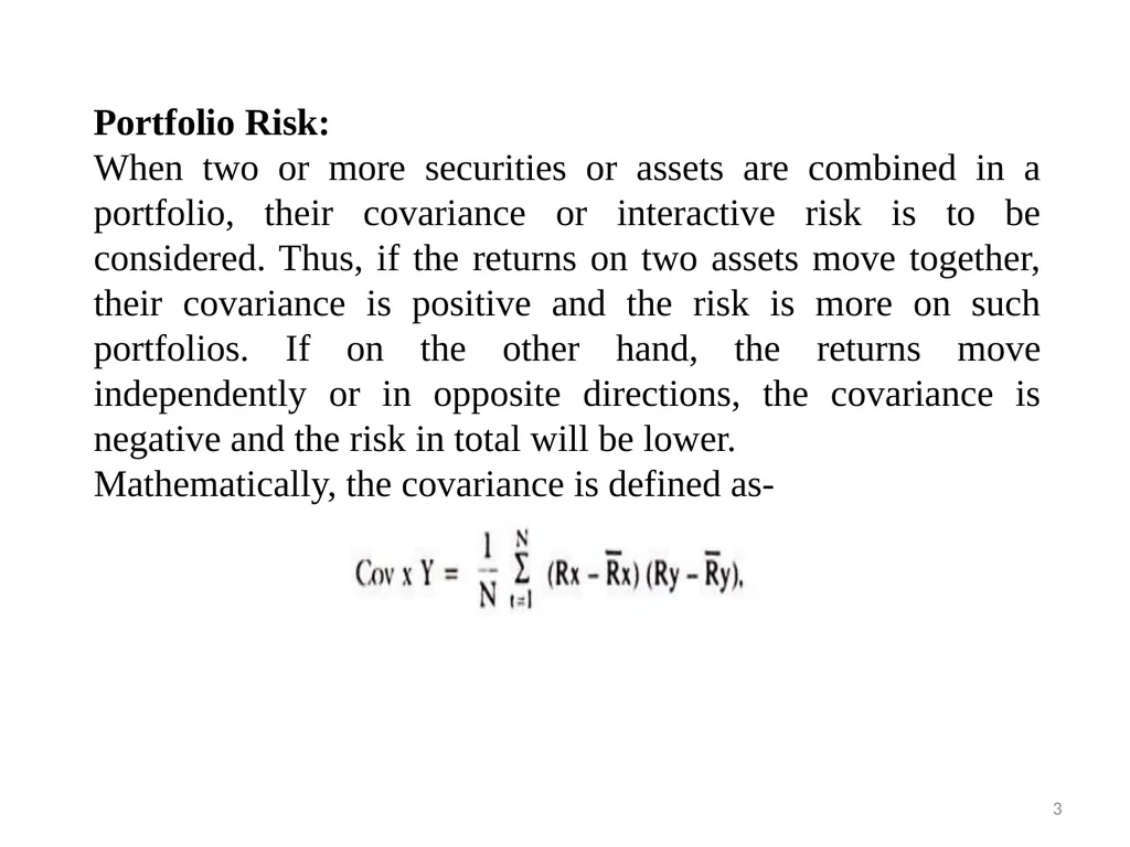
When two or more securities or assets are combined in a portfolio, their covariance or interactive risk is to be considered. Thus, if the returns on two assets move together, their covariance is positive and the risk is more on such portfolios. If on the other hand, the returns move independently or in opposite directions, the covariance is negative and the risk in total will be lower.
Mathematically, the covariance is defined as- 3<br>
slide4. To choose the best portfolio from a number of possible portfolios, each with different return and risk, two separate decisions are to be made,.
Determination of a set of efficient portfolios.
Selection of the best portfolio out of the efficient set. 4<br>
slide5. Efficient frontier and Capital Market Line (CML)
An efficient portfolio is one that produces the highest expected return for any given level of risk. Markowitz showed how to find the frontier of risk and returns for stocks. Only portfolios on the frontier are efficient. Sharpe added the riskless asset return and noted that returns on a line connecting rrf and the tangency point on the efficient frontier was also “feasible” in the sense that portfolios consisting of some of the riskless asset and some of the market portfolio could be developed. The introduction of a risk-free asset in the portfolio changes the Markowitz efficient frontier into a straight line. He called that straight efficient frontier line the Capital Market Line (CML), and he used indifference curves to show how investors with different degrees of risk aversion would choose portfolios with different mixes of stocks and the riskless asset. Investors who are not at all averse to risk could borrow and buy stocks on margin, and thus move out the CML beyond the tangency point. Since the line is straight, the math implies that any two assets falling on this line will be perfectly positively correlated with each other. 5<br>
slide6. Determining the efficient set
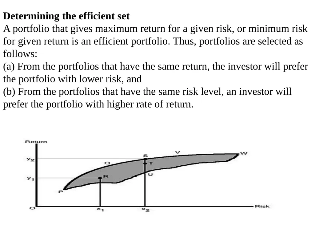
A portfolio that gives maximum return for a given risk, or minimum risk for given return is an efficient portfolio. Thus, portfolios are selected as follows:
(a) From the portfolios that have the same return, the investor will prefer the portfolio with lower risk, and
(b) From the portfolios that have the same risk level, an investor will prefer the portfolio with higher rate of return. 6<br>
slide7. As the investor is rational, they would like to have higher return. And as they are risk averse, they want to have lower risk. In Figure 1, the shaded area PVWP includes all the possible securities an investor can invest in. The efficient portfolios are the ones that lie on the boundary of PQVW. For example, at risk level x2, there are three portfolios S, T, U. But portfolio S is called the efficient portfolio as it has the highest return, y2, compared to T and U[needs dot]. All the portfolios that lie on the boundary of PQVW are efficient portfolios for a given risk level. 7<br>
slide8. The boundary PQVW is called the Efficient Frontier. All portfolios that lie below the Efficient Frontier are not good enough because the return would be lower for the given risk. Portfolios that lie to the right of the Efficient Frontier would not be good enough, as there is higher risk for a given rate of return. All portfolios lying on the boundary of PQVW are called Efficient Portfolios. The Efficient Frontier is the same for all investors, as all investors want maximum return with the lowest possible risk and they are risk averse. 8<br>
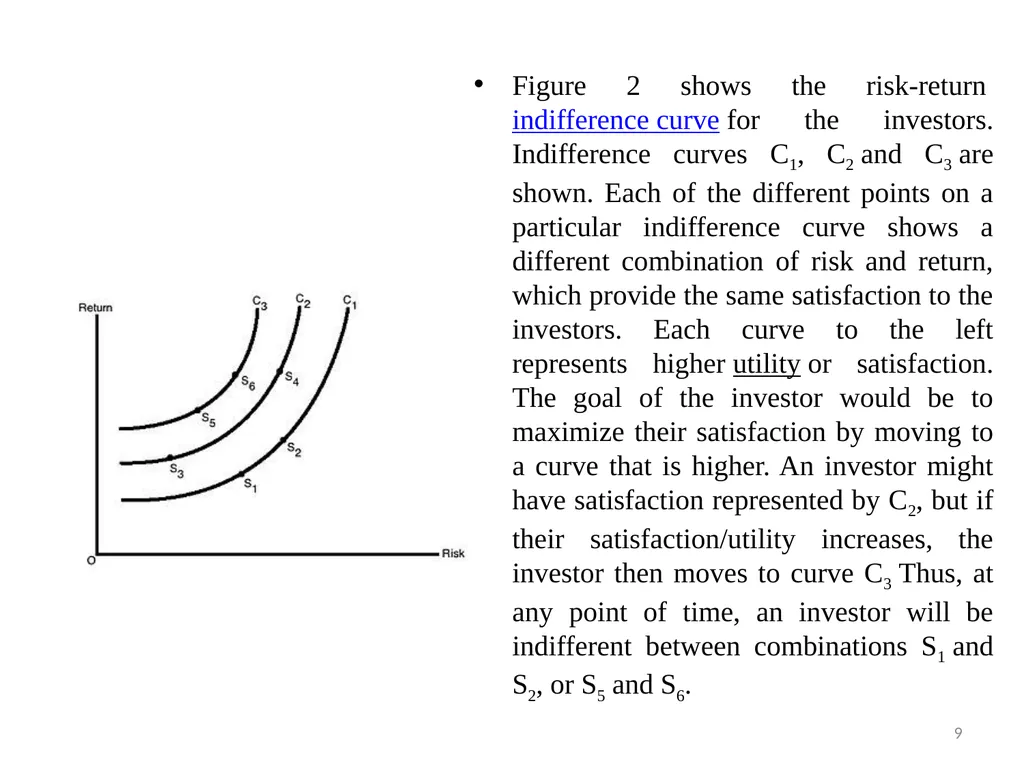
slide9. Figure 2 shows the risk-return indifference curve for the investors. Indifference curves C1, C2 and C3 are shown. Each of the different points on a particular indifference curve shows a different combination of risk and return, which provide the same satisfaction to the investors. Each curve to the left represents higher utility or satisfaction. The goal of the investor would be to maximize their satisfaction by moving to a curve that is higher. An investor might have satisfaction represented by C2, but if their satisfaction/utility increases, the investor then moves to curve C3 Thus, at any point of time, an investor will be indifferent between combinations S1 and S2, or S5 and S6. 9<br>
slide10. The investor's optimal portfolio is found at the point of tangency of the efficient frontier with the indifference curve. This point marks the highest level of satisfaction the investor can obtain. 10<br>
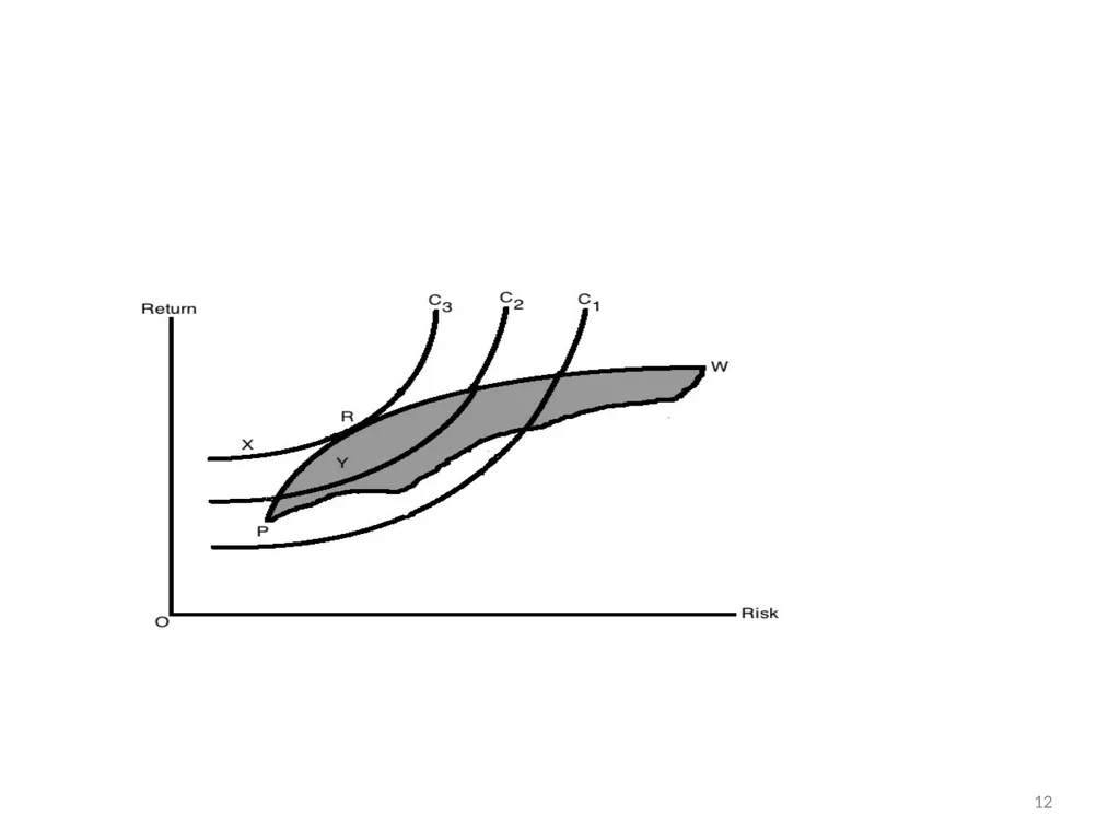
slide11. The investor's optimal portfolio is found at the point of tangency of the efficient frontier with the indifference curve. This point marks the highest level of satisfaction the investor can obtain. This is shown in Figure 3. R is the point where the efficient frontier is tangent to indifference curve C3, and is also an efficient portfolio. With this portfolio, the investor will get highest satisfaction as well as best risk-return combination (a portfolio that provides the highest possible return for a given amount of risk). Any other portfolio, say X, isn't the optimal portfolio even though it lies on the same indifference curve as it is outside the feasible portfolio available in the market. Portfolio Y is also not optimal as it does not lie on the best feasible indifference curve, even though it is a feasible market portfolio. Another investor having other sets of indifference curves might have some different portfolio 11<br>
slide12. 12<br>
slide13. 13<br>
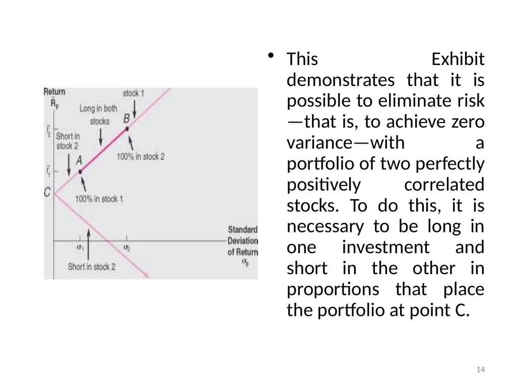
slide14. This Exhibit demonstrates that it is possible to eliminate risk—that is, to achieve zero variance—with a portfolio of two perfectly positively correlated stocks. To do this, it is necessary to be long in one investment and short in the other in proportions that place the portfolio at point C. 14<br>
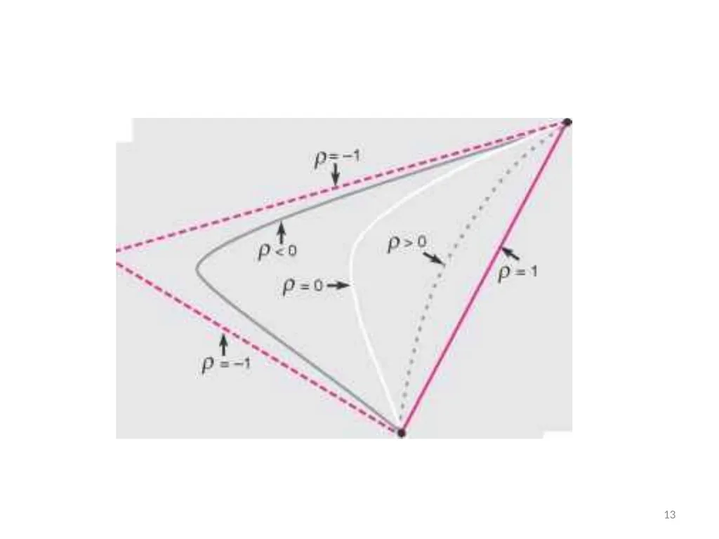
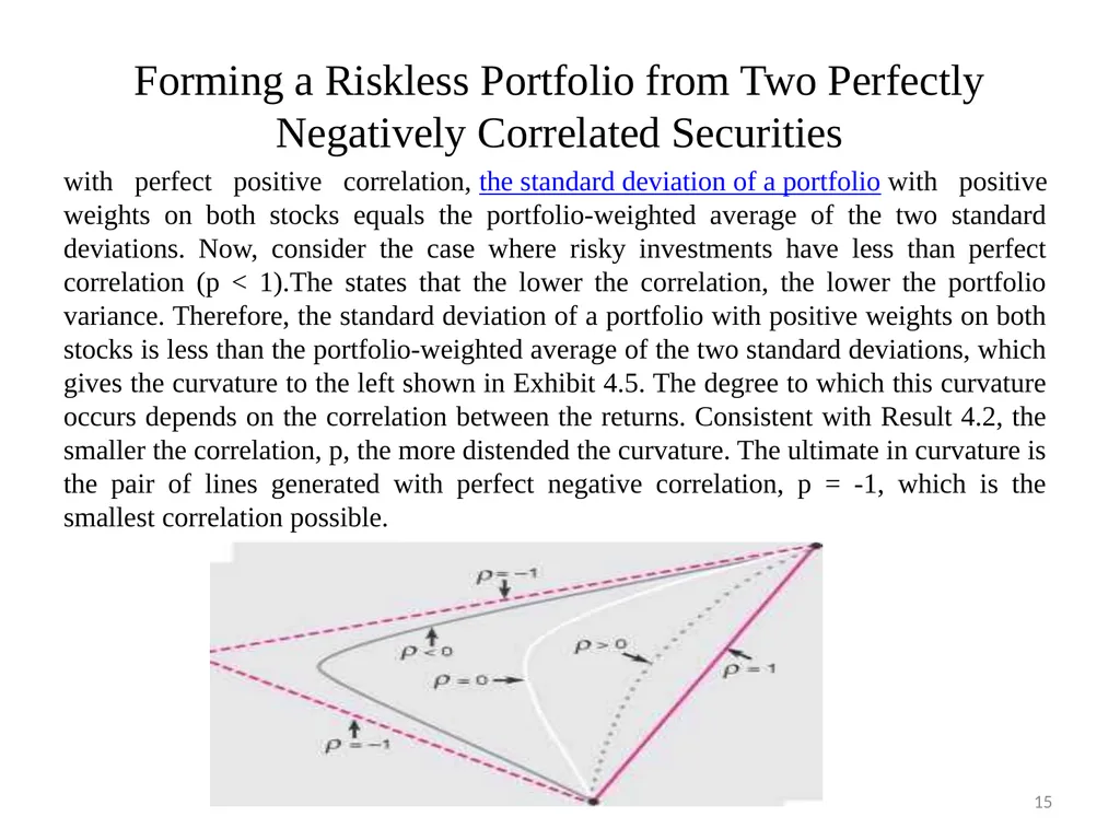
slide15. Forming a Riskless Portfolio from Two Perfectly Negatively Correlated Securities with perfect positive correlation, the standard deviation of a portfolio with positive weights on both stocks equals the portfolio-weighted average of the two standard deviations. Now, consider the case where risky investments have less than perfect correlation (p < 1).The states that the lower the correlation, the lower the portfolio variance. Therefore, the standard deviation of a portfolio with positive weights on both stocks is less than the portfolio-weighted average of the two standard deviations, which gives the curvature to the left shown in Exhibit 4.5. The degree to which this curvature occurs depends on the correlation between the returns. Consistent with Result 4.2, the smaller the correlation, p, the more distended the curvature. The ultimate in curvature is the pair of lines generated with perfect negative correlation, p = -1, which is the smallest correlation possible. 15<br>
slide16. An optimal stock portfolio refers to a stock portfolio that incorporates the stocks configured in such a manner that they yield the optimal return statistically possible at a given level of risk accepted by an investor. The modern portfolio theory stresses on the optimal portfolio concept by assuming that the investors try to minimize risk obsessively while looking for the highest return possible. As per this theory, investors should make rational decisions for achieving maximum returns at their acceptable level of risk.
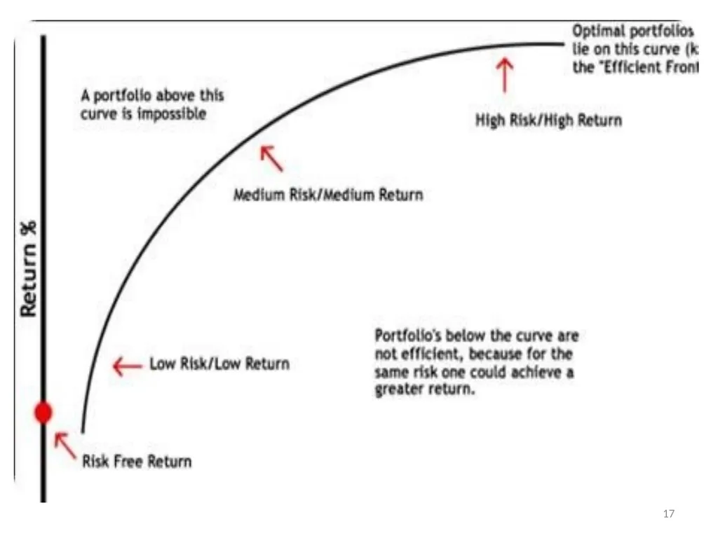
The working of the optimal portfolio can be easily understood by looking at the chart below. The optimal-risk portfolio is generally found in the middle of the curve. If one goes further higher up the curve, it will mean taking more risk proportionately for achieving lower incremental return. Similarly if one goes at lower end of the curve, it will mean low risk/low return portfolios. 16<br>
slide17. 17<br>
slide18. Sources and Types of Risk Sources of Risk:
Interest rate risk
Market risk
Inflation risk
Business risk
Financial risk
Liquidity risk
Exchange rate risk
Country risk
Broad Types:
Systematic/Market Risk
Non-systematic/Non-market/Company-specific Risk 18<br>
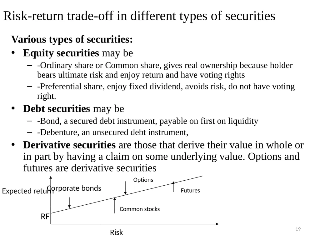
slide19. Risk-return trade-off in different types of securities Various types of securities:
Equity securities may be
-Ordinary share or Common share, gives real ownership because holder bears ultimate risk and enjoy return and have voting rights
-Preferential share, enjoy fixed dividend, avoids risk, do not have voting right.
Debt securities may be
-Bond, a secured debt instrument, payable on first on liquidity
-Debenture, an unsecured debt instrument,
Derivative securities are those that derive their value in whole or in part by having a claim on some underlying value. Options and futures are derivative securities Corporate bonds Common stocks Options Futures RF Expected return Risk 19<br>
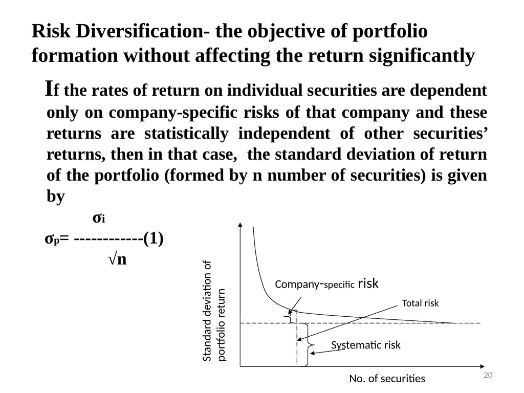
slide20. Risk Diversification- the objective of portfolio formation without affecting the return significantly If the rates of return on individual securities are dependent only on company-specific risks of that company and these returns are statistically independent of other securities’ returns, then in that case, the standard deviation of return of the portfolio (formed by n number of securities) is given by
σi
σp= ------------(1)
√n Standard deviation of portfolio return No. of securities Systematic risk Company-specific risk Total risk 20<br>
slide21. Risk Diversification Risk diversification is the key to the management of portfolio risk, because it allows investors to significantly lower the portfolio risk without adversely affecting return.
Diversification types:
Random or naive diversification
Efficient diversification 21<br>
slide22. Random or naive diversification: It refers to the act of randomly diversifying without regard to relevant investment characteristics such as expected return and industry classification. An investor simply selects relatively large number of securities randomly.
Unfortunately, in such case, the benefits of random diversification do not continue as we add more securities, the reduction becomes smaller and smaller. 22<br>
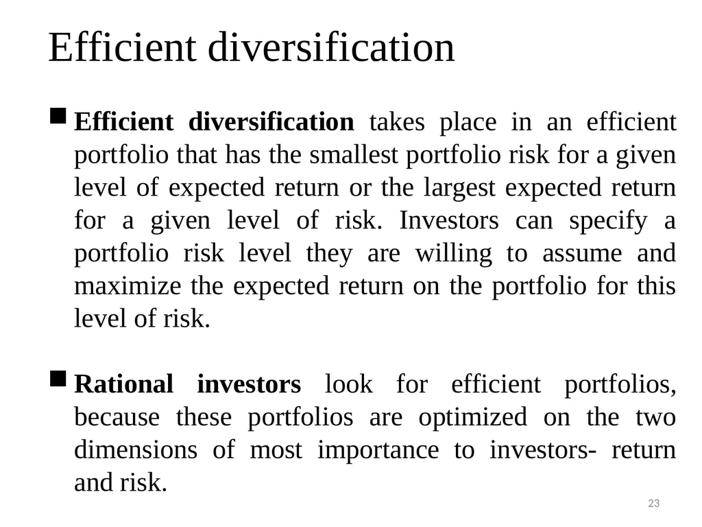
slide23. Efficient diversification Efficient diversification takes place in an efficient portfolio that has the smallest portfolio risk for a given level of expected return or the largest expected return for a given level of risk. Investors can specify a portfolio risk level they are willing to assume and maximize the expected return on the portfolio for this level of risk.
Rational investors look for efficient portfolios, because these portfolios are optimized on the two dimensions of most importance to investors- return and risk. 23<br>
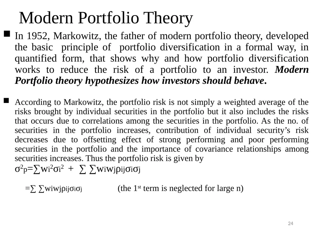
slide24. Modern Portfolio Theory In 1952, Markowitz, the father of modern portfolio theory, developed the basic principle of portfolio diversification in a formal way, in quantified form, that shows why and how portfolio diversification works to reduce the risk of a portfolio to an investor. Modern Portfolio theory hypothesizes how investors should behave.
According to Markowitz, the portfolio risk is not simply a weighted average of the risks brought by individual securities in the portfolio but it also includes the risks that occurs due to correlations among the securities in the portfolio. As the no. of securities in the portfolio increases, contribution of individual security’s risk decreases due to offsetting effect of strong performing and poor performing securities in the portfolio and the importance of covariance relationships among securities increases. Thus the portfolio risk is given by
σ2p=∑wi2σi2 + ∑ ∑wiwjρijσiσj
=∑ ∑wiwjρijσiσj (the 1st term is neglected for large n) 24<br>
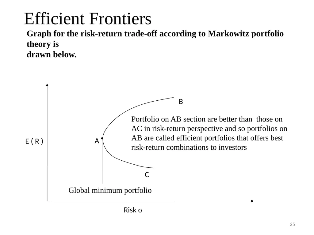
slide25. Efficient Frontiers Risk σ E ( R ) A Global minimum portfolio C B Portfolio on AB section are better than those on AC in risk-return perspective and so portfolios on AB are called efficient portfolios that offers best risk-return combinations to investors Graph for the risk-return trade-off according to Markowitz portfolio theory is
drawn below. 25<br>
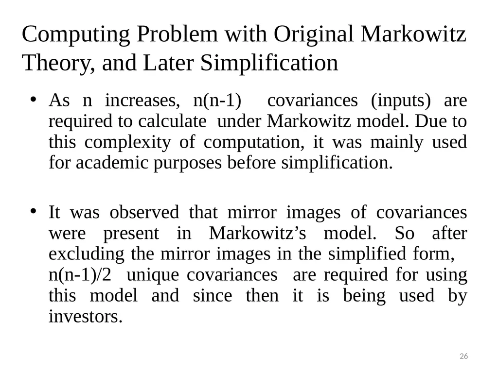
slide26. Computing Problem with Original Markowitz Theory, and Later Simplification As n increases, n(n-1) covariances (inputs) are required to calculate under Markowitz model. Due to this complexity of computation, it was mainly used for academic purposes before simplification.
It was observed that mirror images of covariances were present in Markowitz’s model. So after excluding the mirror images in the simplified form, n(n-1)/2 unique covariances are required for using this model and since then it is being used by investors. 26<br>
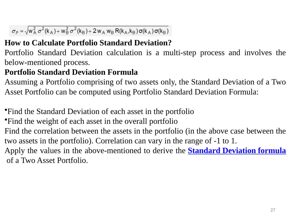
slide27. How to Calculate Portfolio Standard Deviation?
Portfolio Standard Deviation calculation is a multi-step process and involves the below-mentioned process.
Portfolio Standard Deviation Formula
Assuming a Portfolio comprising of two assets only, the Standard Deviation of a Two Asset Portfolio can be computed using Portfolio Standard Deviation Formula:
Find the Standard Deviation of each asset in the portfolio
Find the weight of each asset in the overall portfolio
Find the correlation between the assets in the portfolio (in the above case between the two assets in the portfolio). Correlation can vary in the range of -1 to 1.
Apply the values in the above-mentioned to derive the Standard Deviation formula of a Two Asset Portfolio. 27<br>
slide2. Unit II<br>
slide3. Portfolio Risk:
When two or more securities or assets are combined in a portfolio, their covariance or interactive risk is to be considered. Thus, if the returns on two assets move together, their covariance is positive and the risk is more on such portfolios. If on the other hand, the returns move independently or in opposite directions, the covariance is negative and the risk in total will be lower.
Mathematically, the covariance is defined as- 3<br>
slide4. To choose the best portfolio from a number of possible portfolios, each with different return and risk, two separate decisions are to be made,.
Determination of a set of efficient portfolios.
Selection of the best portfolio out of the efficient set. 4<br>
slide5. Efficient frontier and Capital Market Line (CML)
An efficient portfolio is one that produces the highest expected return for any given level of risk. Markowitz showed how to find the frontier of risk and returns for stocks. Only portfolios on the frontier are efficient. Sharpe added the riskless asset return and noted that returns on a line connecting rrf and the tangency point on the efficient frontier was also “feasible” in the sense that portfolios consisting of some of the riskless asset and some of the market portfolio could be developed. The introduction of a risk-free asset in the portfolio changes the Markowitz efficient frontier into a straight line. He called that straight efficient frontier line the Capital Market Line (CML), and he used indifference curves to show how investors with different degrees of risk aversion would choose portfolios with different mixes of stocks and the riskless asset. Investors who are not at all averse to risk could borrow and buy stocks on margin, and thus move out the CML beyond the tangency point. Since the line is straight, the math implies that any two assets falling on this line will be perfectly positively correlated with each other. 5<br>
slide6. Determining the efficient set
A portfolio that gives maximum return for a given risk, or minimum risk for given return is an efficient portfolio. Thus, portfolios are selected as follows:
(a) From the portfolios that have the same return, the investor will prefer the portfolio with lower risk, and
(b) From the portfolios that have the same risk level, an investor will prefer the portfolio with higher rate of return. 6<br>
slide7. As the investor is rational, they would like to have higher return. And as they are risk averse, they want to have lower risk. In Figure 1, the shaded area PVWP includes all the possible securities an investor can invest in. The efficient portfolios are the ones that lie on the boundary of PQVW. For example, at risk level x2, there are three portfolios S, T, U. But portfolio S is called the efficient portfolio as it has the highest return, y2, compared to T and U[needs dot]. All the portfolios that lie on the boundary of PQVW are efficient portfolios for a given risk level. 7<br>
slide8. The boundary PQVW is called the Efficient Frontier. All portfolios that lie below the Efficient Frontier are not good enough because the return would be lower for the given risk. Portfolios that lie to the right of the Efficient Frontier would not be good enough, as there is higher risk for a given rate of return. All portfolios lying on the boundary of PQVW are called Efficient Portfolios. The Efficient Frontier is the same for all investors, as all investors want maximum return with the lowest possible risk and they are risk averse. 8<br>
slide9. Figure 2 shows the risk-return indifference curve for the investors. Indifference curves C1, C2 and C3 are shown. Each of the different points on a particular indifference curve shows a different combination of risk and return, which provide the same satisfaction to the investors. Each curve to the left represents higher utility or satisfaction. The goal of the investor would be to maximize their satisfaction by moving to a curve that is higher. An investor might have satisfaction represented by C2, but if their satisfaction/utility increases, the investor then moves to curve C3 Thus, at any point of time, an investor will be indifferent between combinations S1 and S2, or S5 and S6. 9<br>
slide10. The investor's optimal portfolio is found at the point of tangency of the efficient frontier with the indifference curve. This point marks the highest level of satisfaction the investor can obtain. 10<br>
slide11. The investor's optimal portfolio is found at the point of tangency of the efficient frontier with the indifference curve. This point marks the highest level of satisfaction the investor can obtain. This is shown in Figure 3. R is the point where the efficient frontier is tangent to indifference curve C3, and is also an efficient portfolio. With this portfolio, the investor will get highest satisfaction as well as best risk-return combination (a portfolio that provides the highest possible return for a given amount of risk). Any other portfolio, say X, isn't the optimal portfolio even though it lies on the same indifference curve as it is outside the feasible portfolio available in the market. Portfolio Y is also not optimal as it does not lie on the best feasible indifference curve, even though it is a feasible market portfolio. Another investor having other sets of indifference curves might have some different portfolio 11<br>
slide12. 12<br>
slide13. 13<br>
slide14. This Exhibit demonstrates that it is possible to eliminate risk—that is, to achieve zero variance—with a portfolio of two perfectly positively correlated stocks. To do this, it is necessary to be long in one investment and short in the other in proportions that place the portfolio at point C. 14<br>
slide15. Forming a Riskless Portfolio from Two Perfectly Negatively Correlated Securities with perfect positive correlation, the standard deviation of a portfolio with positive weights on both stocks equals the portfolio-weighted average of the two standard deviations. Now, consider the case where risky investments have less than perfect correlation (p < 1).The states that the lower the correlation, the lower the portfolio variance. Therefore, the standard deviation of a portfolio with positive weights on both stocks is less than the portfolio-weighted average of the two standard deviations, which gives the curvature to the left shown in Exhibit 4.5. The degree to which this curvature occurs depends on the correlation between the returns. Consistent with Result 4.2, the smaller the correlation, p, the more distended the curvature. The ultimate in curvature is the pair of lines generated with perfect negative correlation, p = -1, which is the smallest correlation possible. 15<br>
slide16. An optimal stock portfolio refers to a stock portfolio that incorporates the stocks configured in such a manner that they yield the optimal return statistically possible at a given level of risk accepted by an investor. The modern portfolio theory stresses on the optimal portfolio concept by assuming that the investors try to minimize risk obsessively while looking for the highest return possible. As per this theory, investors should make rational decisions for achieving maximum returns at their acceptable level of risk.
The working of the optimal portfolio can be easily understood by looking at the chart below. The optimal-risk portfolio is generally found in the middle of the curve. If one goes further higher up the curve, it will mean taking more risk proportionately for achieving lower incremental return. Similarly if one goes at lower end of the curve, it will mean low risk/low return portfolios. 16<br>
slide17. 17<br>
slide18. Sources and Types of Risk Sources of Risk:
Interest rate risk
Market risk
Inflation risk
Business risk
Financial risk
Liquidity risk
Exchange rate risk
Country risk
Broad Types:
Systematic/Market Risk
Non-systematic/Non-market/Company-specific Risk 18<br>
slide19. Risk-return trade-off in different types of securities Various types of securities:
Equity securities may be
-Ordinary share or Common share, gives real ownership because holder bears ultimate risk and enjoy return and have voting rights
-Preferential share, enjoy fixed dividend, avoids risk, do not have voting right.
Debt securities may be
-Bond, a secured debt instrument, payable on first on liquidity
-Debenture, an unsecured debt instrument,
Derivative securities are those that derive their value in whole or in part by having a claim on some underlying value. Options and futures are derivative securities Corporate bonds Common stocks Options Futures RF Expected return Risk 19<br>
slide20. Risk Diversification- the objective of portfolio formation without affecting the return significantly If the rates of return on individual securities are dependent only on company-specific risks of that company and these returns are statistically independent of other securities’ returns, then in that case, the standard deviation of return of the portfolio (formed by n number of securities) is given by
σi
σp= ------------(1)
√n Standard deviation of portfolio return No. of securities Systematic risk Company-specific risk Total risk 20<br>
slide21. Risk Diversification Risk diversification is the key to the management of portfolio risk, because it allows investors to significantly lower the portfolio risk without adversely affecting return.
Diversification types:
Random or naive diversification
Efficient diversification 21<br>
slide22. Random or naive diversification: It refers to the act of randomly diversifying without regard to relevant investment characteristics such as expected return and industry classification. An investor simply selects relatively large number of securities randomly.
Unfortunately, in such case, the benefits of random diversification do not continue as we add more securities, the reduction becomes smaller and smaller. 22<br>
slide23. Efficient diversification Efficient diversification takes place in an efficient portfolio that has the smallest portfolio risk for a given level of expected return or the largest expected return for a given level of risk. Investors can specify a portfolio risk level they are willing to assume and maximize the expected return on the portfolio for this level of risk.
Rational investors look for efficient portfolios, because these portfolios are optimized on the two dimensions of most importance to investors- return and risk. 23<br>
slide24. Modern Portfolio Theory In 1952, Markowitz, the father of modern portfolio theory, developed the basic principle of portfolio diversification in a formal way, in quantified form, that shows why and how portfolio diversification works to reduce the risk of a portfolio to an investor. Modern Portfolio theory hypothesizes how investors should behave.
According to Markowitz, the portfolio risk is not simply a weighted average of the risks brought by individual securities in the portfolio but it also includes the risks that occurs due to correlations among the securities in the portfolio. As the no. of securities in the portfolio increases, contribution of individual security’s risk decreases due to offsetting effect of strong performing and poor performing securities in the portfolio and the importance of covariance relationships among securities increases. Thus the portfolio risk is given by
σ2p=∑wi2σi2 + ∑ ∑wiwjρijσiσj
=∑ ∑wiwjρijσiσj (the 1st term is neglected for large n) 24<br>
slide25. Efficient Frontiers Risk σ E ( R ) A Global minimum portfolio C B Portfolio on AB section are better than those on AC in risk-return perspective and so portfolios on AB are called efficient portfolios that offers best risk-return combinations to investors Graph for the risk-return trade-off according to Markowitz portfolio theory is
drawn below. 25<br>
slide26. Computing Problem with Original Markowitz Theory, and Later Simplification As n increases, n(n-1) covariances (inputs) are required to calculate under Markowitz model. Due to this complexity of computation, it was mainly used for academic purposes before simplification.
It was observed that mirror images of covariances were present in Markowitz’s model. So after excluding the mirror images in the simplified form, n(n-1)/2 unique covariances are required for using this model and since then it is being used by investors. 26<br>
slide27. How to Calculate Portfolio Standard Deviation?
Portfolio Standard Deviation calculation is a multi-step process and involves the below-mentioned process.
Portfolio Standard Deviation Formula
Assuming a Portfolio comprising of two assets only, the Standard Deviation of a Two Asset Portfolio can be computed using Portfolio Standard Deviation Formula:
Find the Standard Deviation of each asset in the portfolio
Find the weight of each asset in the overall portfolio
Find the correlation between the assets in the portfolio (in the above case between the two assets in the portfolio). Correlation can vary in the range of -1 to 1.
Apply the values in the above-mentioned to derive the Standard Deviation formula of a Two Asset Portfolio. 27<br>