
Real Options Analysis Lecture No. 44 Chapter 13
Description: Real Options Analysis Lecture No. 44 Chapter 13 Contemporary Engineering Economics Copyright 2016 What Is Real About Real Options? Concept: Any corporate investment decision to invest and or divest real assets is simply an option,
Related Topics
Download Presentation
"Real Options Analysis Lecture No. 44 Chapter 13" is the property of its rightful owner. Permission is granted to download and print the materials on this website for personal, non-commercial use only, and to display it on your personal computer provided you do not modify the materials and that you retain all copyright notices contained in the materials. By downloading content from our website, you accept the terms of this agreement.
Presentation Transcript
slide1. Real Options Analysis Lecture No. 44
Chapter 13
Contemporary Engineering Economics
Copyright © 2016<br>
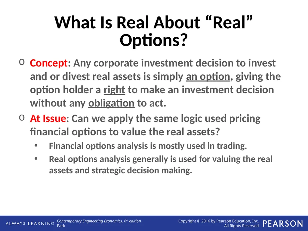
slide2. What Is Real About “Real” Options? Concept: Any corporate investment decision to invest and or divest real assets is simply an option, giving the option holder a right to make an investment decision without any obligation to act.
At Issue: Can we apply the same logic used pricing financial options to value the real assets?
Financial options analysis is mostly used in trading.
Real options analysis generally is used for valuing the real assets and strategic decision making.<br>
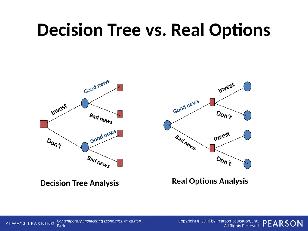
slide3. Decision Tree vs. Real Options Invest Good news Bad news Don’t Good news Bad news Decision Tree Analysis Real Options Analysis Invest Don’t Invest Don’t Good news Bad news<br>
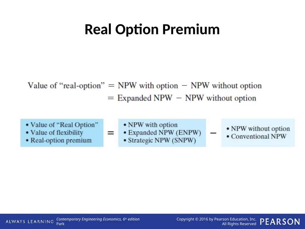
slide4. Real Option Premium<br>
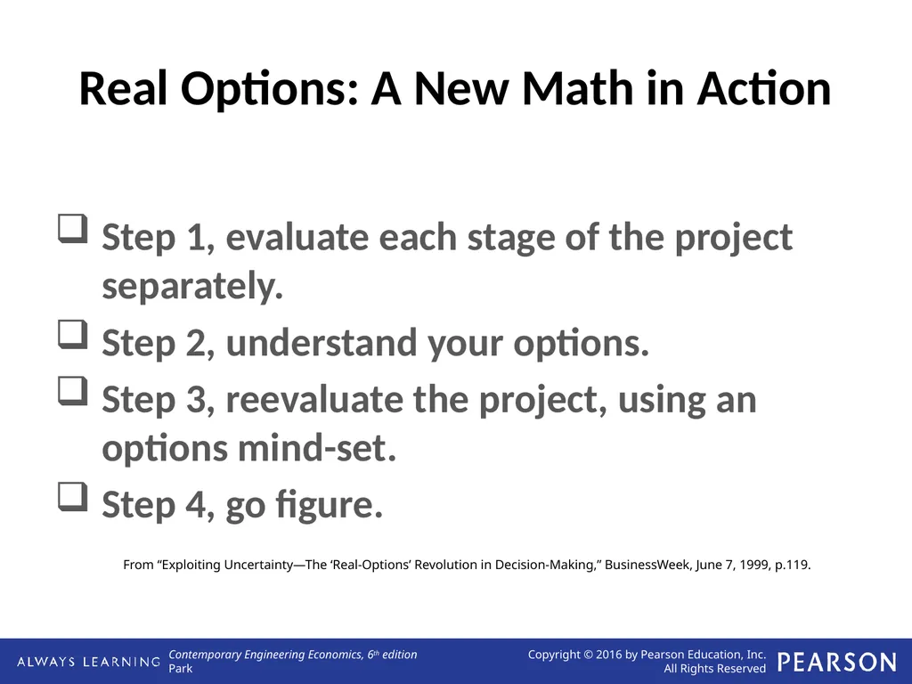
slide5. Real Options: A New Math in Action Step 1, evaluate each stage of the project separately.
Step 2, understand your options.
Step 3, reevaluate the project, using an options mind-set.
Step 4, go figure. From “Exploiting Uncertainty—The ‘Real-Options’ Revolution in Decision-Making,” BusinessWeek, June 7, 1999, p.119.<br>
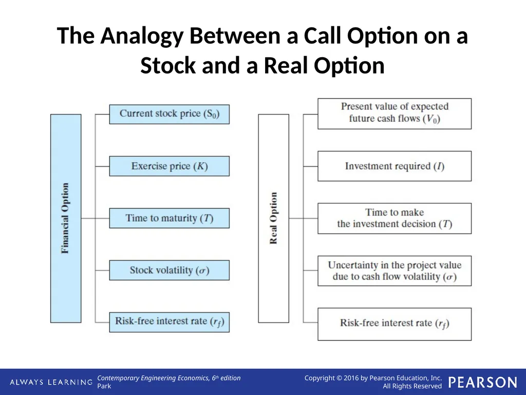
slide6. The Analogy Between a Call Option on a Stock and a Real Option<br>
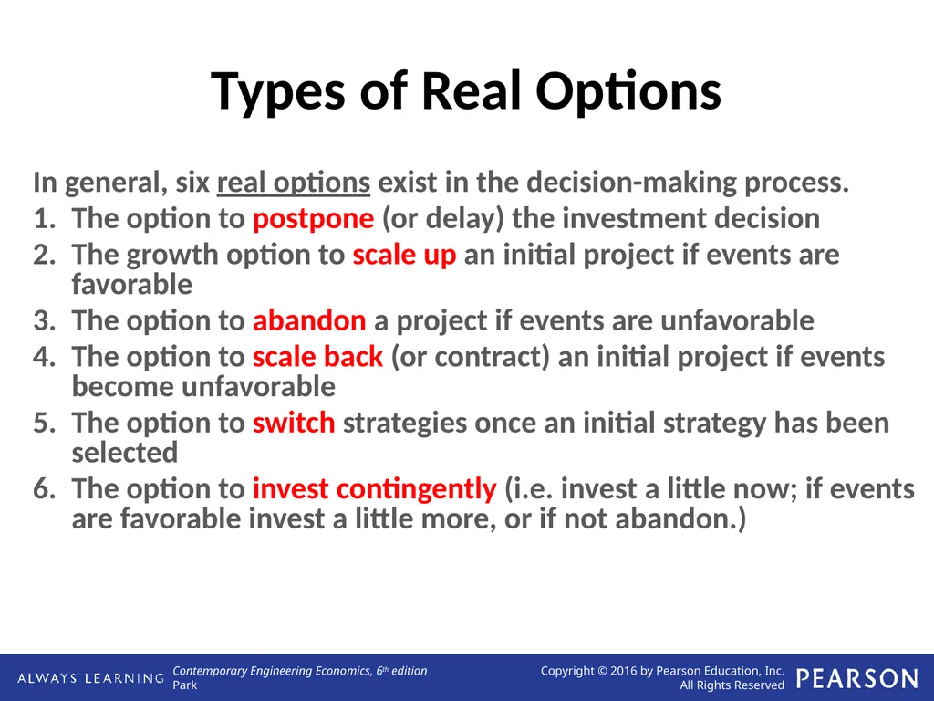
slide7. Types of Real Options In general, six real options exist in the decision-making process.
The option to postpone (or delay) the investment decision
The growth option to scale up an initial project if events are favorable
The option to abandon a project if events are unfavorable
The option to scale back (or contract) an initial project if events become unfavorable
The option to switch strategies once an initial strategy has been selected
The option to invest contingently (i.e. invest a little now; if events are favorable invest a little more, or if not abandon.)<br>
slide8. Delay Option The decision-maker (DM) does not always need to initiate a project immediately.
The DM has the option to postpone the investment decision due to:
Uncertainty in market demand
Uncertainty in market timing
Uncertainty in market input/output prices
Real options analysis (ROA) values the flexibility to postpone the investment decision.<br>
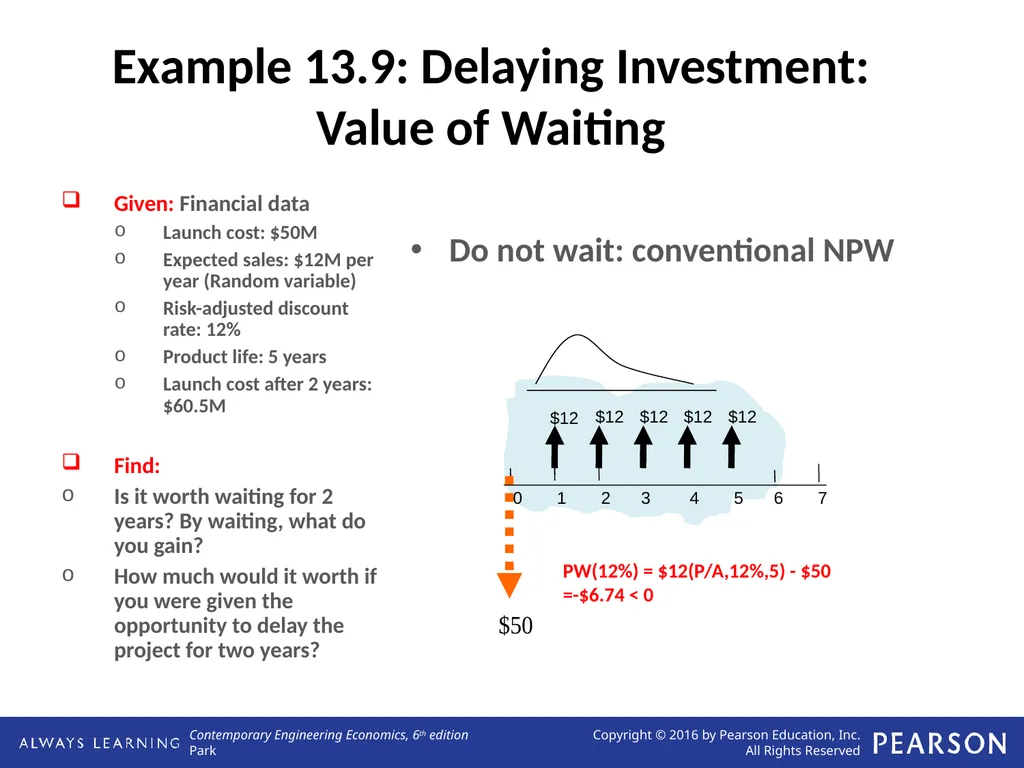
slide9. Example 13.9: Delaying Investment: Value of Waiting Do not wait: conventional NPW Given: Financial data
Launch cost: $50M
Expected sales: $12M per year (Random variable)
Risk-adjusted discount rate: 12%
Product life: 5 years
Launch cost after 2 years: $60.5M
Find:
Is it worth waiting for 2 years? By waiting, what do you gain?
How much would it worth if you were given the opportunity to delay the project for two years? 0 1 2 3 4 5 6 7 $12 $12 $12 $12 $12 PW(12%) = $12(P/A,12%,5) - $50
=-$6.74 < 0<br>
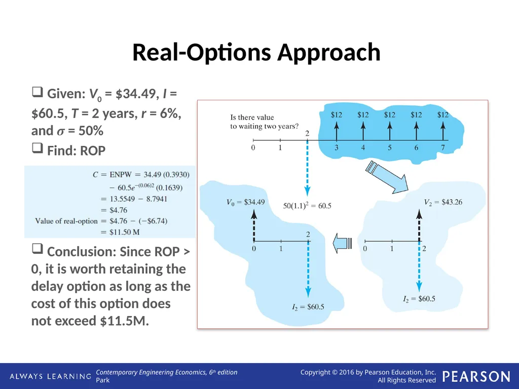
slide10. Real-Options Approach Given: V0 = $34.49, I = $60.5, T = 2 years, r = 6%, and σ = 50%
Find: ROP
Conclusion: Since ROP > 0, it is worth retaining the delay option as long as the cost of this option does not exceed $11.5M.<br>
slide11. Economic Interpretation What exactly does the $4.76 M delay value imply?
Assume the firm has 10 projects. One of these 10 projects is this digital phone investment. Assume the other 9 projects have a net present value of $100 M.
Standard NPV: The value of the firm using standard NPV would still be $100 M including the digital phone project because the project has a negative NPV today and would not be accepted.
Delay Option: If the option to invest in the digital phones is included in the firm evaluation, then the value of the firm is $104.76 M. Therefore, the delay option that the firm possesses is worth an additional $4.76 M.<br>
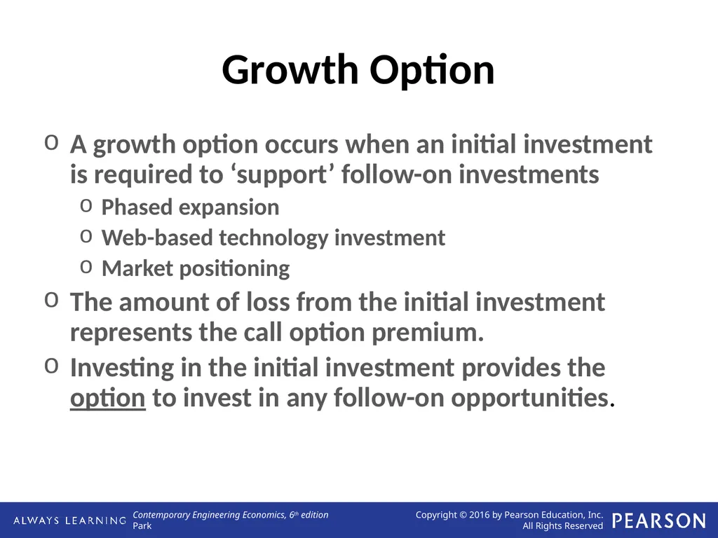
slide12. Growth Option A growth option occurs when an initial investment is required to ‘support’ follow-on investments
Phased expansion
Web-based technology investment
Market positioning
The amount of loss from the initial investment represents the call option premium.
Investing in the initial investment provides the option to invest in any follow-on opportunities.<br>
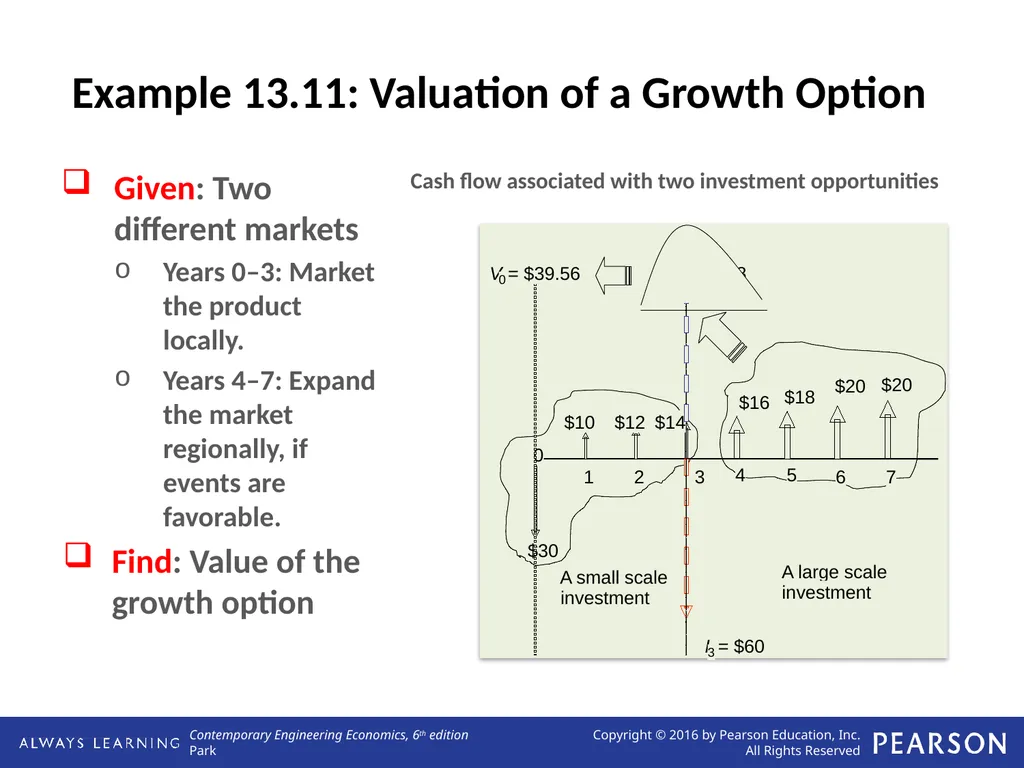
slide13. Example 13.11: Valuation of a Growth Option Cash flow associated with two investment opportunities Given: Two different markets
Years 0–3: Market the product locally.
Years 4–7: Expand the market regionally, if events are favorable.
Find: Value of the growth option<br>
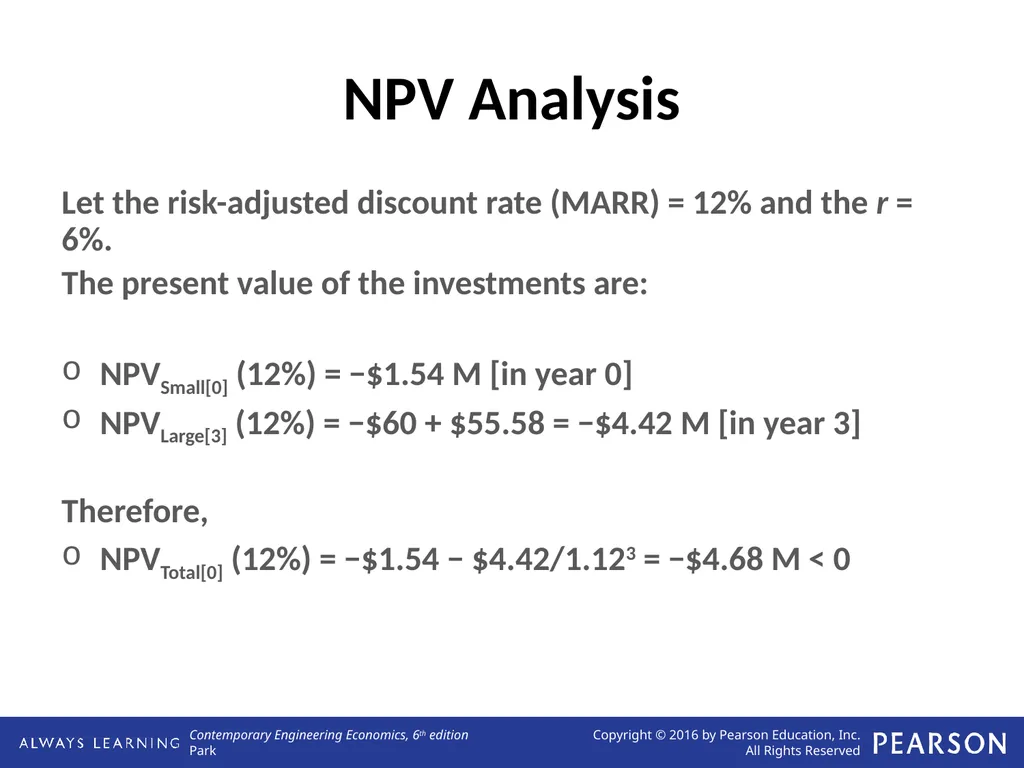
slide14. NPV Analysis Let the risk-adjusted discount rate (MARR) = 12% and the r = 6%.
The present value of the investments are:
NPVSmall[0] (12%) = −$1.54 M [in year 0]
NPVLarge[3] (12%) = −$60 + $55.58 = −$4.42 M [in year 3]
Therefore,
NPVTotal[0] (12%) = −$1.54 − $4.42/1.123 = −$4.68 M < 0<br>
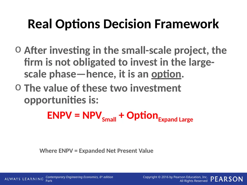
slide15. Real Options Decision Framework After investing in the small-scale project, the firm is not obligated to invest in the large-scale phase—hence, it is an option.
The value of these two investment opportunities is:
ENPV = NPVSmall + OptionExpand Large
Where ENPV = Expanded Net Present Value<br>
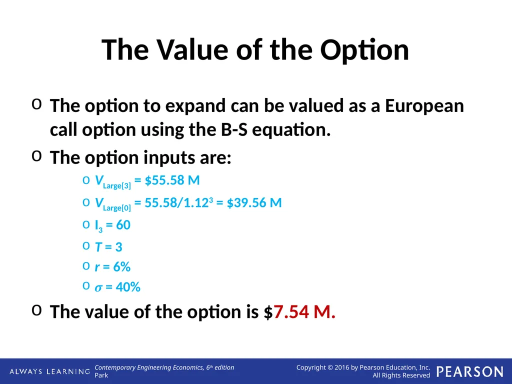
slide16. The Value of the Option The option to expand can be valued as a European call option using the B-S equation.
The option inputs are:
VLarge[3] = $55.58 M
VLarge[0] = 55.58/1.123 = $39.56 M
I3 = 60
T = 3
r = 6%
σ = 40%
The value of the option is $7.54 M.<br>
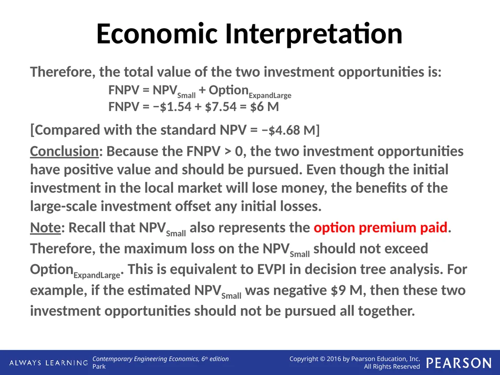
slide17. Economic Interpretation Therefore, the total value of the two investment opportunities is:
FNPV = NPVSmall + OptionExpandLarge
FNPV = −$1.54 + $7.54 = $6 M
[Compared with the standard NPV = −$4.68 M]
Conclusion: Because the FNPV > 0, the two investment opportunities have positive value and should be pursued. Even though the initial investment in the local market will lose money, the benefits of the large-scale investment offset any initial losses.
Note: Recall that NPVSmall also represents the option premium paid. Therefore, the maximum loss on the NPVSmall should not exceed OptionExpandLarge. This is equivalent to EVPI in decision tree analysis. For example, if the estimated NPVSmall was negative $9 M, then these two investment opportunities should not be pursued all together.<br>
slide18. Scale-up Option A firm has the right to scale-up an investment if the initial project is favorable.
A firm has the option to increase investment in a project, in return for increased revenues.
This is just a growth option, but will be valued on a binomial lattice.<br>
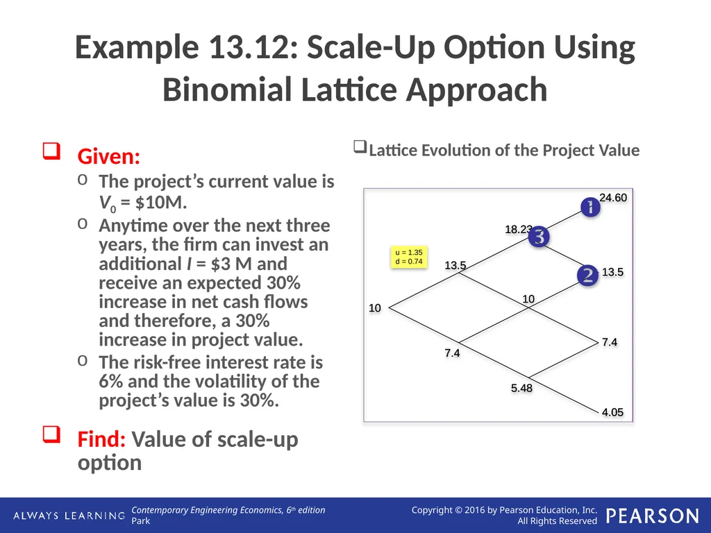
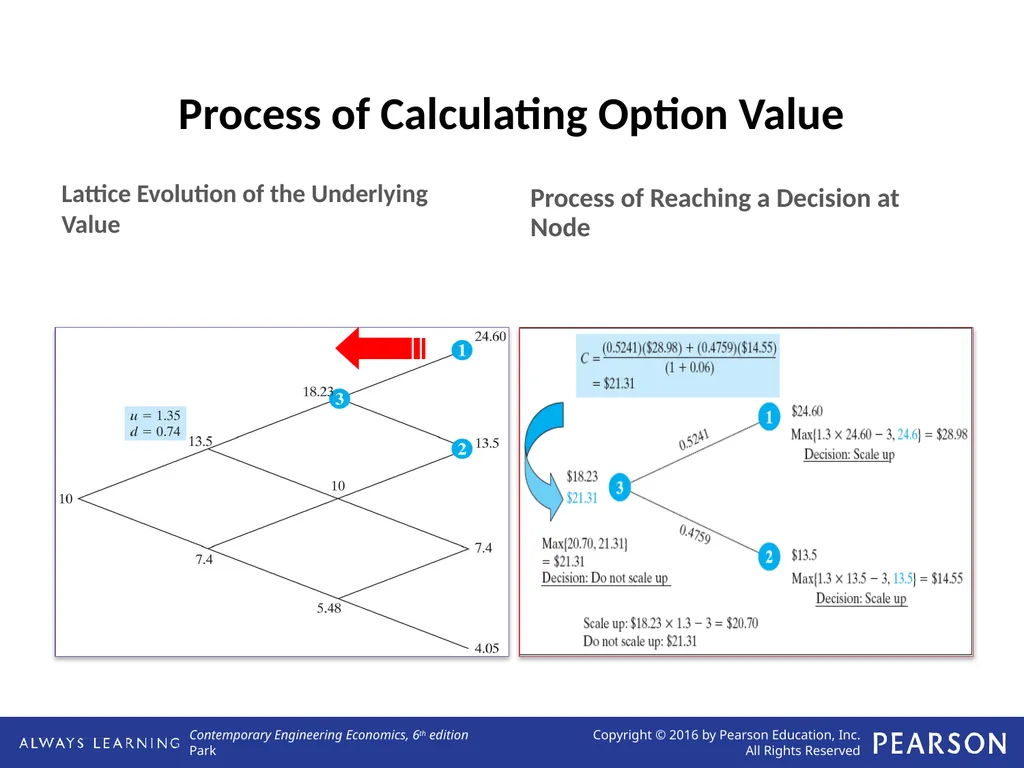
slide19. Example 13.12: Scale-Up Option Using Binomial Lattice Approach Given:
The project’s current value is V0 = $10M.
Anytime over the next three years, the firm can invest an additional I = $3 M and receive an expected 30% increase in net cash flows and therefore, a 30% increase in project value.
The risk-free interest rate is 6% and the volatility of the project’s value is 30%.
Find: Value of scale-up option Lattice Evolution of the Project Value<br>
slide20. Process of Calculating Option Value Lattice Evolution of the Underlying Value Process of Reaching a Decision at Node<br>
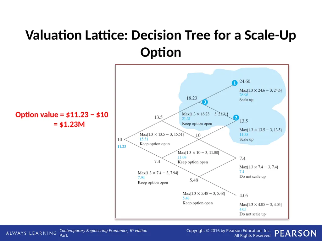
slide21. Valuation Lattice: Decision Tree for a Scale-Up Option Option value = $11.23 − $10
= $1.23M<br>
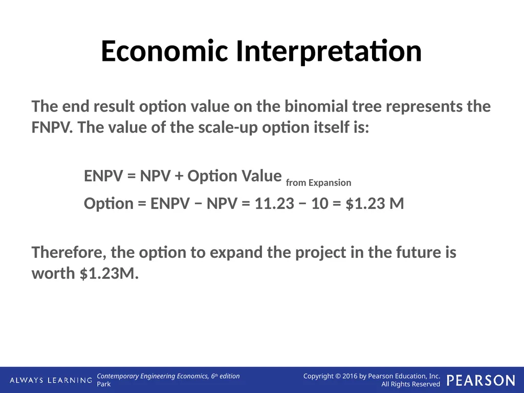
slide22. Economic Interpretation The end result option value on the binomial tree represents the FNPV. The value of the scale-up option itself is:
ENPV = NPV + Option Value from Expansion
Option = ENPV − NPV = 11.23 − 10 = $1.23 M
Therefore, the option to expand the project in the future is worth $1.23M.<br>
slide23. Scale-down Option A firm has the right to scale-down an investment if the initial project is unfavorable.
This is a scaled version of the abandonment option and will be valued on a binomial lattice.<br>
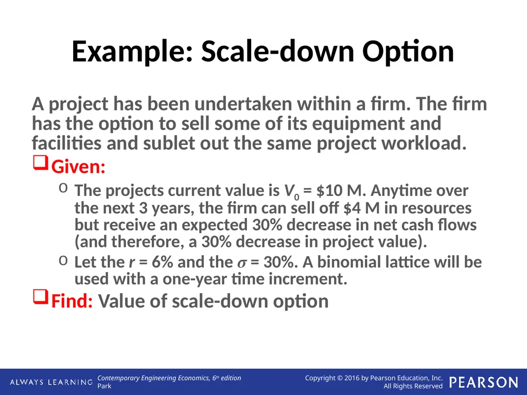
slide24. Example: Scale-down Option A project has been undertaken within a firm. The firm has the option to sell some of its equipment and facilities and sublet out the same project workload.
Given:
The projects current value is V0 = $10 M. Anytime over the next 3 years, the firm can sell off $4 M in resources but receive an expected 30% decrease in net cash flows (and therefore, a 30% decrease in project value).
Let the r = 6% and the σ = 30%. A binomial lattice will be used with a one-year time increment.
Find: Value of scale-down option<br>
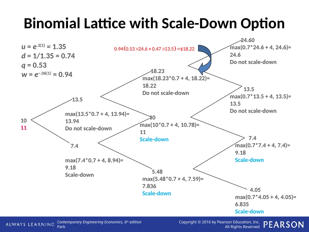
slide25. Binomial Lattice with Scale-Down Option u = e.3(1) = 1.35
d = 1/1.35 = 0.74
q = 0.53
w = e−.06(1) = 0.94 10
11 13.5
max(13.5*0.7 + 4, 13.94)=
13.94
Do not scale-down 7.4
max(7.4*0.7 + 4, 8.94)=
9.18
Scale-down 18.23
max(18.23*0.7 + 4, 18.22)=
18.22
Do not scale-down 24.60
max(0.7*24.6 + 4, 24.6)=
24.6
Do not scale-down 10
max(10*0.7 + 4, 10.78)=
11
Scale-down 13.5
max(0.7*13.5 + 4, 13.5)=
13.5
Do not scale-down 7.4
max(0.7*7.4 + 4, 7.4)=
9.18
Scale-down 5.48
max(5.48*0.7 + 4, 7.59)=
7.836
Scale-down 4.05
max(0.7*4.05 + 4, 4.05)=
6.835
Scale-down<br>
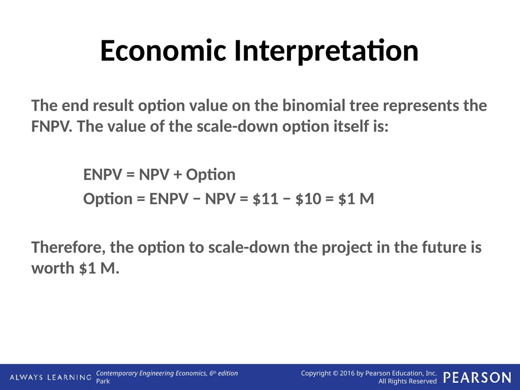
slide26. Economic Interpretation The end result option value on the binomial tree represents the FNPV. The value of the scale-down option itself is:
ENPV = NPV + Option
Option = ENPV − NPV = $11 − $10 = $1 M
Therefore, the option to scale-down the project in the future is worth $1 M.<br>
slide27. Compound Options The value of option depends on the value of another option.
A sequential compound option exists when a project has a multiple phases and later phases depend on the success of earlier phases.
Invest a little, observe results; the option to invest more
Local, regional, national, international
Phased investment
Research & development
Growth opportunities<br>
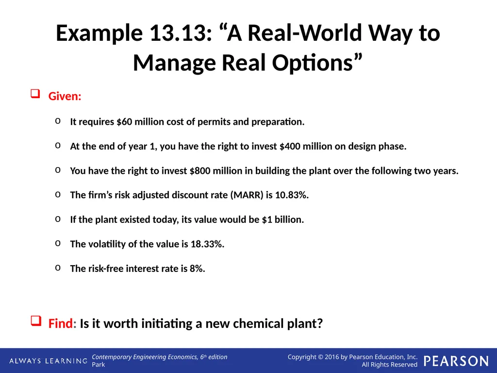
slide28. Example 13.13: “A Real-World Way to Manage Real Options” Given:
It requires $60 million cost of permits and preparation.
At the end of year 1, you have the right to invest $400 million on design phase.
You have the right to invest $800 million in building the plant over the following two years.
The firm’s risk adjusted discount rate (MARR) is 10.83%.
If the plant existed today, its value would be $1 billion.
The volatility of the value is 18.33%.
The risk-free interest rate is 8%.
Find: Is it worth initiating a new chemical plant?<br>
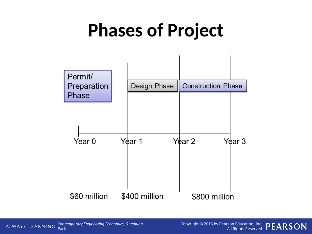
slide29. Phases of Project<br>
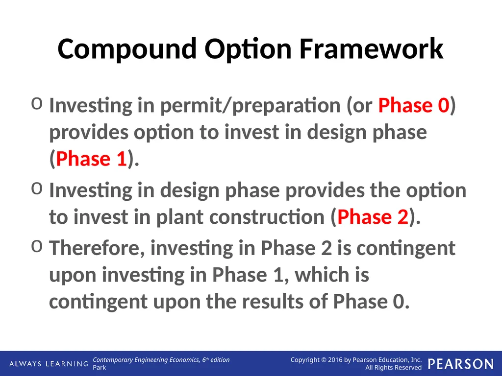
slide30. Compound Option Framework Investing in permit/preparation (or Phase 0) provides option to invest in design phase (Phase 1).
Investing in design phase provides the option to invest in plant construction (Phase 2).
Therefore, investing in Phase 2 is contingent upon investing in Phase 1, which is contingent upon the results of Phase 0.<br>
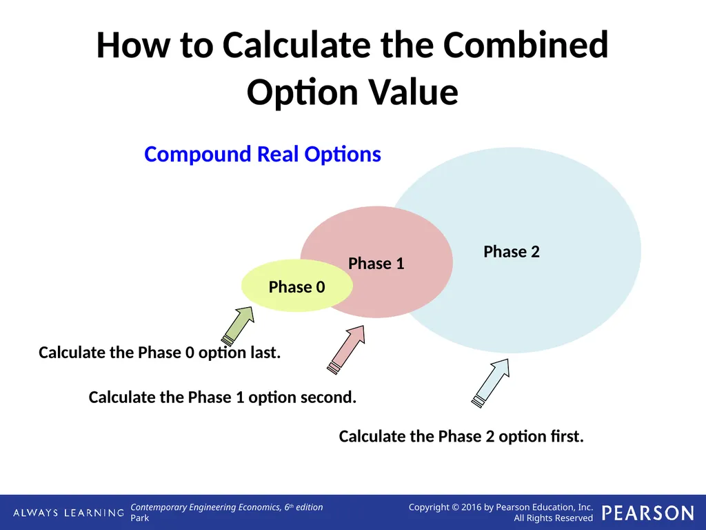
slide31. How to Calculate the Combined Option Value Phase 2 Phase 1 Phase 0 Compound Real Options Calculate the Phase 2 option first. Calculate the Phase 1 option second. Calculate the Phase 0 option last.<br>
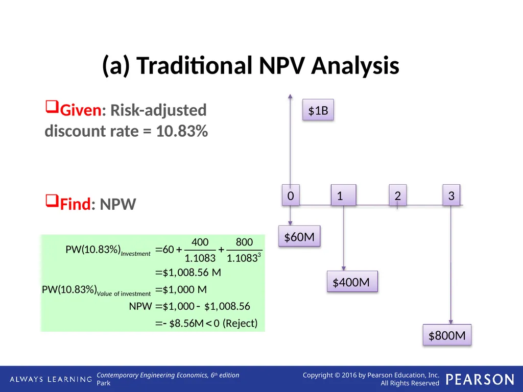
slide32. (a) Traditional NPV Analysis Given: Risk-adjusted discount rate = 10.83%
Find: NPW<br>
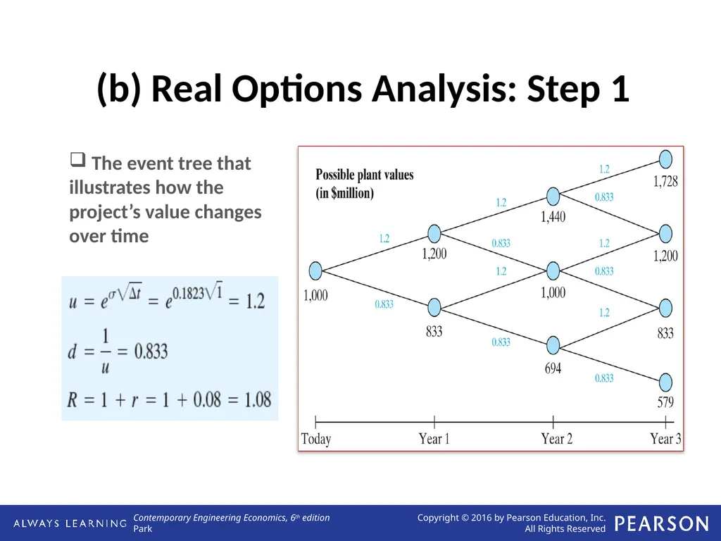
slide33. (b) Real Options Analysis: Step 1 The event tree that illustrates how the project’s value changes over time<br>
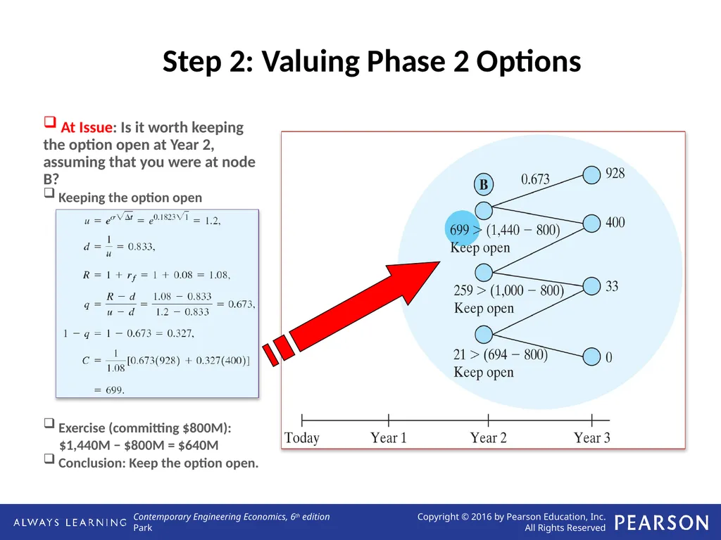
slide34. Step 2: Valuing Phase 2 Options At Issue: Is it worth keeping the option open at Year 2, assuming that you were at node B?
Keeping the option open
Exercise (committing $800M):
$1,440M − $800M = $640M
Conclusion: Keep the option open.<br>
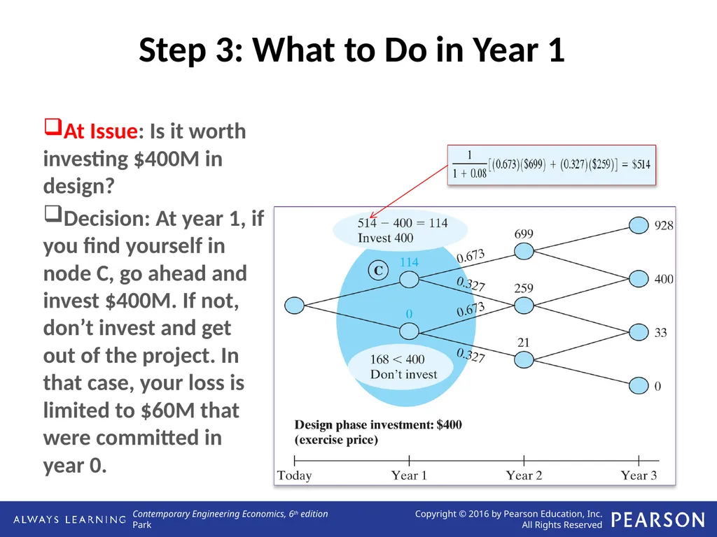
slide35. Step 3: What to Do in Year 1 At Issue: Is it worth investing $400M in design?
Decision: At year 1, if you find yourself in node C, go ahead and invest $400M. If not, don’t invest and get out of the project. In that case, your loss is limited to $60M that were committed in year 0.<br>
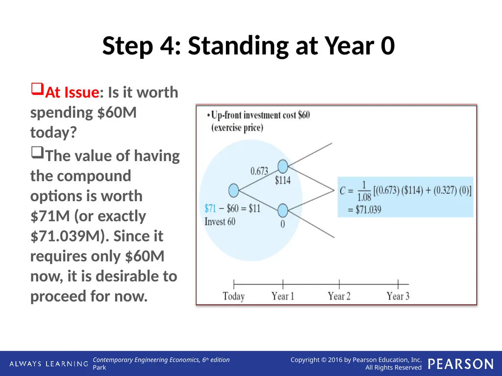
slide36. Step 4: Standing at Year 0 At Issue: Is it worth spending $60M today?
The value of having the compound options is worth $71M (or exactly $71.039M). Since it requires only $60M now, it is desirable to proceed for now.<br>
Chapter 13
Contemporary Engineering Economics
Copyright © 2016<br>
slide2. What Is Real About “Real” Options? Concept: Any corporate investment decision to invest and or divest real assets is simply an option, giving the option holder a right to make an investment decision without any obligation to act.
At Issue: Can we apply the same logic used pricing financial options to value the real assets?
Financial options analysis is mostly used in trading.
Real options analysis generally is used for valuing the real assets and strategic decision making.<br>
slide3. Decision Tree vs. Real Options Invest Good news Bad news Don’t Good news Bad news Decision Tree Analysis Real Options Analysis Invest Don’t Invest Don’t Good news Bad news<br>
slide4. Real Option Premium<br>
slide5. Real Options: A New Math in Action Step 1, evaluate each stage of the project separately.
Step 2, understand your options.
Step 3, reevaluate the project, using an options mind-set.
Step 4, go figure. From “Exploiting Uncertainty—The ‘Real-Options’ Revolution in Decision-Making,” BusinessWeek, June 7, 1999, p.119.<br>
slide6. The Analogy Between a Call Option on a Stock and a Real Option<br>
slide7. Types of Real Options In general, six real options exist in the decision-making process.
The option to postpone (or delay) the investment decision
The growth option to scale up an initial project if events are favorable
The option to abandon a project if events are unfavorable
The option to scale back (or contract) an initial project if events become unfavorable
The option to switch strategies once an initial strategy has been selected
The option to invest contingently (i.e. invest a little now; if events are favorable invest a little more, or if not abandon.)<br>
slide8. Delay Option The decision-maker (DM) does not always need to initiate a project immediately.
The DM has the option to postpone the investment decision due to:
Uncertainty in market demand
Uncertainty in market timing
Uncertainty in market input/output prices
Real options analysis (ROA) values the flexibility to postpone the investment decision.<br>
slide9. Example 13.9: Delaying Investment: Value of Waiting Do not wait: conventional NPW Given: Financial data
Launch cost: $50M
Expected sales: $12M per year (Random variable)
Risk-adjusted discount rate: 12%
Product life: 5 years
Launch cost after 2 years: $60.5M
Find:
Is it worth waiting for 2 years? By waiting, what do you gain?
How much would it worth if you were given the opportunity to delay the project for two years? 0 1 2 3 4 5 6 7 $12 $12 $12 $12 $12 PW(12%) = $12(P/A,12%,5) - $50
=-$6.74 < 0<br>
slide10. Real-Options Approach Given: V0 = $34.49, I = $60.5, T = 2 years, r = 6%, and σ = 50%
Find: ROP
Conclusion: Since ROP > 0, it is worth retaining the delay option as long as the cost of this option does not exceed $11.5M.<br>
slide11. Economic Interpretation What exactly does the $4.76 M delay value imply?
Assume the firm has 10 projects. One of these 10 projects is this digital phone investment. Assume the other 9 projects have a net present value of $100 M.
Standard NPV: The value of the firm using standard NPV would still be $100 M including the digital phone project because the project has a negative NPV today and would not be accepted.
Delay Option: If the option to invest in the digital phones is included in the firm evaluation, then the value of the firm is $104.76 M. Therefore, the delay option that the firm possesses is worth an additional $4.76 M.<br>
slide12. Growth Option A growth option occurs when an initial investment is required to ‘support’ follow-on investments
Phased expansion
Web-based technology investment
Market positioning
The amount of loss from the initial investment represents the call option premium.
Investing in the initial investment provides the option to invest in any follow-on opportunities.<br>
slide13. Example 13.11: Valuation of a Growth Option Cash flow associated with two investment opportunities Given: Two different markets
Years 0–3: Market the product locally.
Years 4–7: Expand the market regionally, if events are favorable.
Find: Value of the growth option<br>
slide14. NPV Analysis Let the risk-adjusted discount rate (MARR) = 12% and the r = 6%.
The present value of the investments are:
NPVSmall[0] (12%) = −$1.54 M [in year 0]
NPVLarge[3] (12%) = −$60 + $55.58 = −$4.42 M [in year 3]
Therefore,
NPVTotal[0] (12%) = −$1.54 − $4.42/1.123 = −$4.68 M < 0<br>
slide15. Real Options Decision Framework After investing in the small-scale project, the firm is not obligated to invest in the large-scale phase—hence, it is an option.
The value of these two investment opportunities is:
ENPV = NPVSmall + OptionExpand Large
Where ENPV = Expanded Net Present Value<br>
slide16. The Value of the Option The option to expand can be valued as a European call option using the B-S equation.
The option inputs are:
VLarge[3] = $55.58 M
VLarge[0] = 55.58/1.123 = $39.56 M
I3 = 60
T = 3
r = 6%
σ = 40%
The value of the option is $7.54 M.<br>
slide17. Economic Interpretation Therefore, the total value of the two investment opportunities is:
FNPV = NPVSmall + OptionExpandLarge
FNPV = −$1.54 + $7.54 = $6 M
[Compared with the standard NPV = −$4.68 M]
Conclusion: Because the FNPV > 0, the two investment opportunities have positive value and should be pursued. Even though the initial investment in the local market will lose money, the benefits of the large-scale investment offset any initial losses.
Note: Recall that NPVSmall also represents the option premium paid. Therefore, the maximum loss on the NPVSmall should not exceed OptionExpandLarge. This is equivalent to EVPI in decision tree analysis. For example, if the estimated NPVSmall was negative $9 M, then these two investment opportunities should not be pursued all together.<br>
slide18. Scale-up Option A firm has the right to scale-up an investment if the initial project is favorable.
A firm has the option to increase investment in a project, in return for increased revenues.
This is just a growth option, but will be valued on a binomial lattice.<br>
slide19. Example 13.12: Scale-Up Option Using Binomial Lattice Approach Given:
The project’s current value is V0 = $10M.
Anytime over the next three years, the firm can invest an additional I = $3 M and receive an expected 30% increase in net cash flows and therefore, a 30% increase in project value.
The risk-free interest rate is 6% and the volatility of the project’s value is 30%.
Find: Value of scale-up option Lattice Evolution of the Project Value<br>
slide20. Process of Calculating Option Value Lattice Evolution of the Underlying Value Process of Reaching a Decision at Node<br>
slide21. Valuation Lattice: Decision Tree for a Scale-Up Option Option value = $11.23 − $10
= $1.23M<br>
slide22. Economic Interpretation The end result option value on the binomial tree represents the FNPV. The value of the scale-up option itself is:
ENPV = NPV + Option Value from Expansion
Option = ENPV − NPV = 11.23 − 10 = $1.23 M
Therefore, the option to expand the project in the future is worth $1.23M.<br>
slide23. Scale-down Option A firm has the right to scale-down an investment if the initial project is unfavorable.
This is a scaled version of the abandonment option and will be valued on a binomial lattice.<br>
slide24. Example: Scale-down Option A project has been undertaken within a firm. The firm has the option to sell some of its equipment and facilities and sublet out the same project workload.
Given:
The projects current value is V0 = $10 M. Anytime over the next 3 years, the firm can sell off $4 M in resources but receive an expected 30% decrease in net cash flows (and therefore, a 30% decrease in project value).
Let the r = 6% and the σ = 30%. A binomial lattice will be used with a one-year time increment.
Find: Value of scale-down option<br>
slide25. Binomial Lattice with Scale-Down Option u = e.3(1) = 1.35
d = 1/1.35 = 0.74
q = 0.53
w = e−.06(1) = 0.94 10
11 13.5
max(13.5*0.7 + 4, 13.94)=
13.94
Do not scale-down 7.4
max(7.4*0.7 + 4, 8.94)=
9.18
Scale-down 18.23
max(18.23*0.7 + 4, 18.22)=
18.22
Do not scale-down 24.60
max(0.7*24.6 + 4, 24.6)=
24.6
Do not scale-down 10
max(10*0.7 + 4, 10.78)=
11
Scale-down 13.5
max(0.7*13.5 + 4, 13.5)=
13.5
Do not scale-down 7.4
max(0.7*7.4 + 4, 7.4)=
9.18
Scale-down 5.48
max(5.48*0.7 + 4, 7.59)=
7.836
Scale-down 4.05
max(0.7*4.05 + 4, 4.05)=
6.835
Scale-down<br>
slide26. Economic Interpretation The end result option value on the binomial tree represents the FNPV. The value of the scale-down option itself is:
ENPV = NPV + Option
Option = ENPV − NPV = $11 − $10 = $1 M
Therefore, the option to scale-down the project in the future is worth $1 M.<br>
slide27. Compound Options The value of option depends on the value of another option.
A sequential compound option exists when a project has a multiple phases and later phases depend on the success of earlier phases.
Invest a little, observe results; the option to invest more
Local, regional, national, international
Phased investment
Research & development
Growth opportunities<br>
slide28. Example 13.13: “A Real-World Way to Manage Real Options” Given:
It requires $60 million cost of permits and preparation.
At the end of year 1, you have the right to invest $400 million on design phase.
You have the right to invest $800 million in building the plant over the following two years.
The firm’s risk adjusted discount rate (MARR) is 10.83%.
If the plant existed today, its value would be $1 billion.
The volatility of the value is 18.33%.
The risk-free interest rate is 8%.
Find: Is it worth initiating a new chemical plant?<br>
slide29. Phases of Project<br>
slide30. Compound Option Framework Investing in permit/preparation (or Phase 0) provides option to invest in design phase (Phase 1).
Investing in design phase provides the option to invest in plant construction (Phase 2).
Therefore, investing in Phase 2 is contingent upon investing in Phase 1, which is contingent upon the results of Phase 0.<br>
slide31. How to Calculate the Combined Option Value Phase 2 Phase 1 Phase 0 Compound Real Options Calculate the Phase 2 option first. Calculate the Phase 1 option second. Calculate the Phase 0 option last.<br>
slide32. (a) Traditional NPV Analysis Given: Risk-adjusted discount rate = 10.83%
Find: NPW<br>
slide33. (b) Real Options Analysis: Step 1 The event tree that illustrates how the project’s value changes over time<br>
slide34. Step 2: Valuing Phase 2 Options At Issue: Is it worth keeping the option open at Year 2, assuming that you were at node B?
Keeping the option open
Exercise (committing $800M):
$1,440M − $800M = $640M
Conclusion: Keep the option open.<br>
slide35. Step 3: What to Do in Year 1 At Issue: Is it worth investing $400M in design?
Decision: At year 1, if you find yourself in node C, go ahead and invest $400M. If not, don’t invest and get out of the project. In that case, your loss is limited to $60M that were committed in year 0.<br>
slide36. Step 4: Standing at Year 0 At Issue: Is it worth spending $60M today?
The value of having the compound options is worth $71M (or exactly $71.039M). Since it requires only $60M now, it is desirable to proceed for now.<br>