
Structure conditioning strategy and toy model A.


Description: Structure conditioning strategy and toy model A. Degiovanni, J. Giner Navarro, W. Wuensch 02.04.2014 CLIC RF Structure Development Meeting Outline PART 1: conditioning strategy picture of the current conditioning strategy proposal of
Related Topics
Download Presentation
"Structure conditioning strategy and toy model A." is the property of its rightful owner. Permission is granted to download and print the materials on this website for personal, non-commercial use only, and to display it on your personal computer provided you do not modify the materials and that you retain all copyright notices contained in the materials. By downloading content from our website, you accept the terms of this agreement.
Presentation Transcript
slide1. Structure conditioning strategy
and toy model A. Degiovanni, J. Giner Navarro, W. Wuensch
02.04.2014
CLIC RF Structure Development Meeting<br>
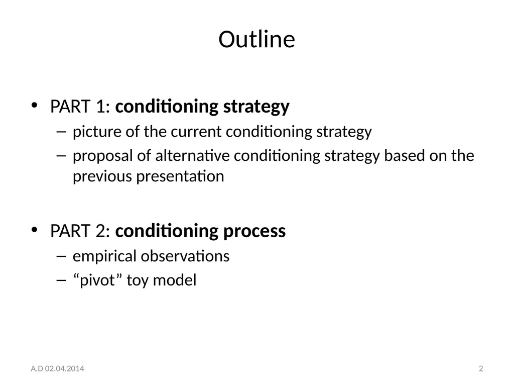
slide2. Outline PART 1: conditioning strategy
picture of the current conditioning strategy
proposal of alternative conditioning strategy based on the previous presentation
PART 2: conditioning process
empirical observations
“pivot” toy model A.D 02.04.2014 2<br>
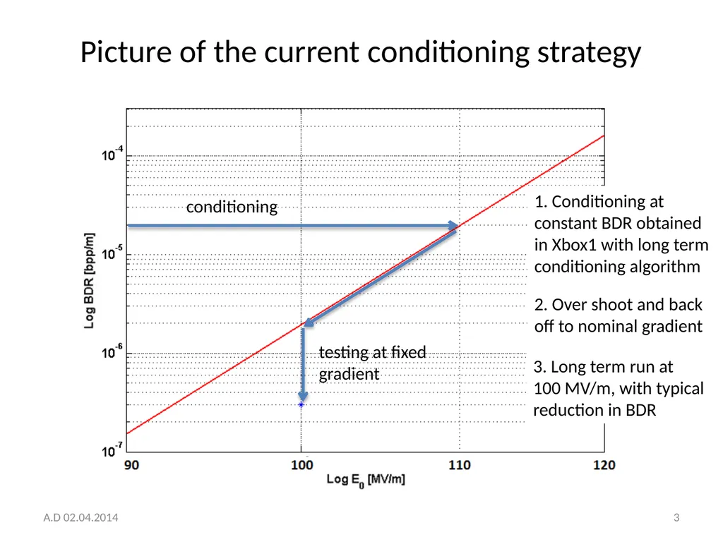
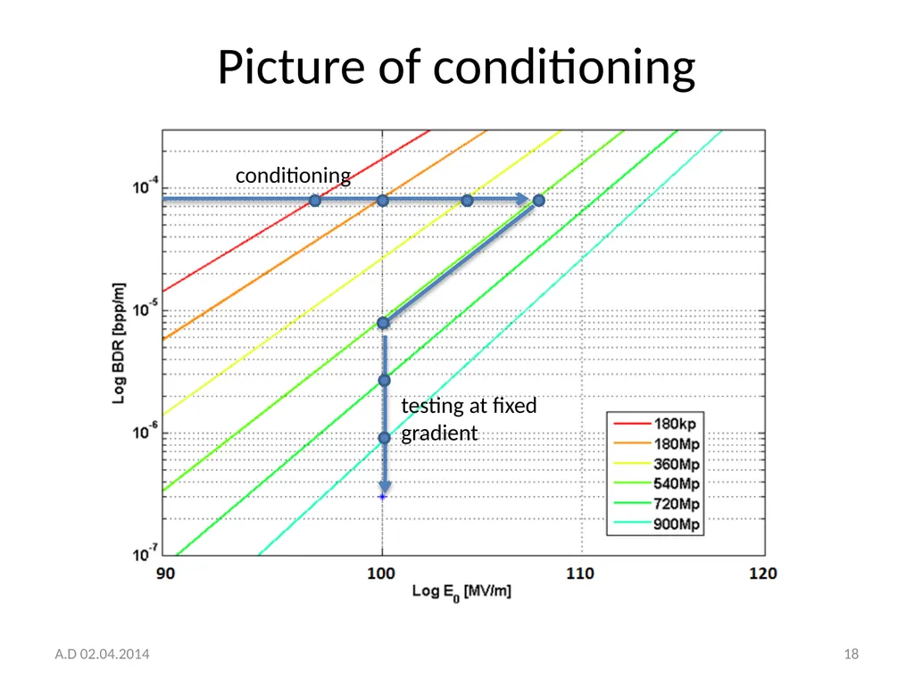
slide3. Picture of the current conditioning strategy 3 1. Conditioning at constant BDR obtained in Xbox1 with long term conditioning algorithm 2. Over shoot and back off to nominal gradient 3. Long term run at 100 MV/m, with typical reduction in BDR A.D 02.04.2014<br>
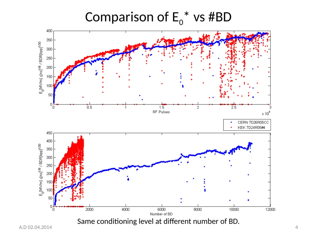
slide4. Comparison of E0* vs #BD 4 A.D 02.04.2014 Same conditioning level at different number of BD.<br>
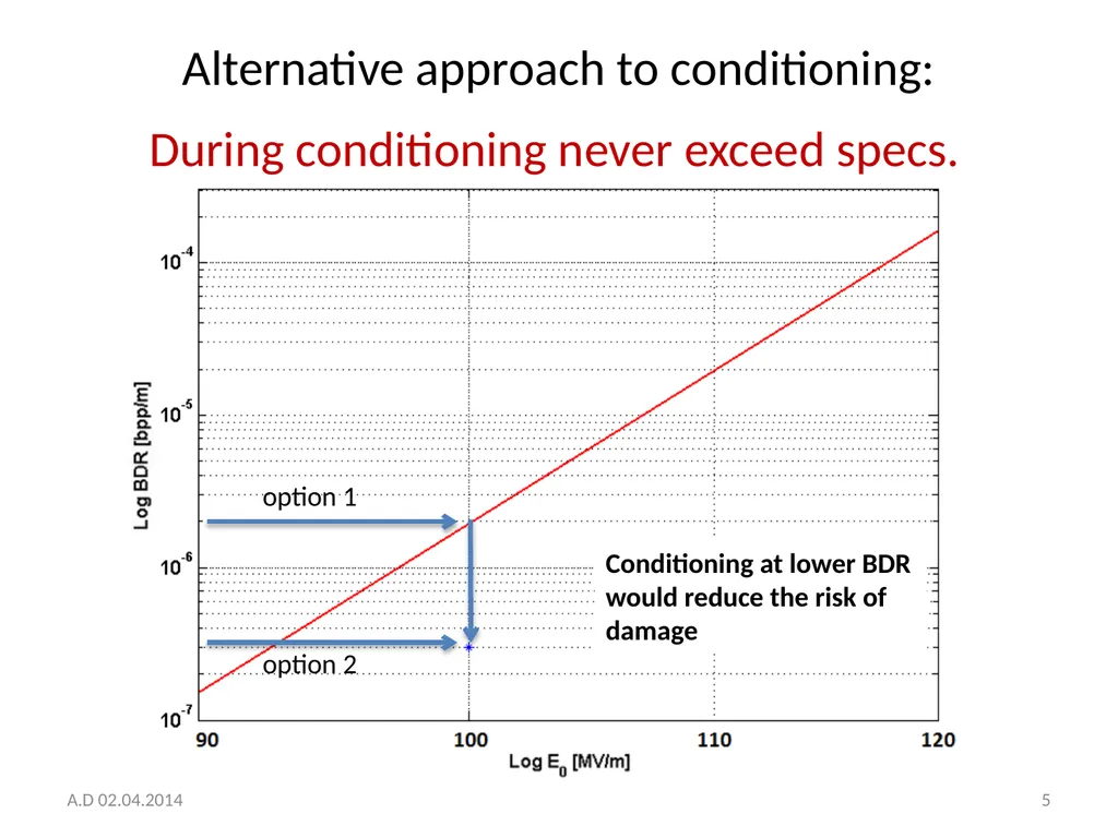
slide5. Alternative approach to conditioning: A.D 02.04.2014 5 During conditioning never exceed specs. option 1 option 2<br>
slide6. PART 2: conditioning process Empirical observations about “conditioning”:
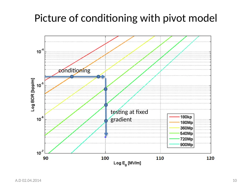
during conditioning we can reach higher gradients at a fixed BDR,
at a fixed gradient, the BDR drops with time.
Some questions:
can we go to infinitely high gradients? probably not
can we think to reduce the BDR to extremely low values?
is the dependence between BDR and E0 fixed in time?
What is presented here is a “toy-model”, a graphical way of thinking about how conditioning works, to trigger the discussion A.D 02.04.2014 6<br>
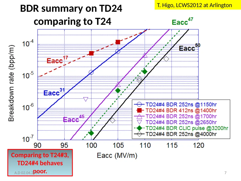
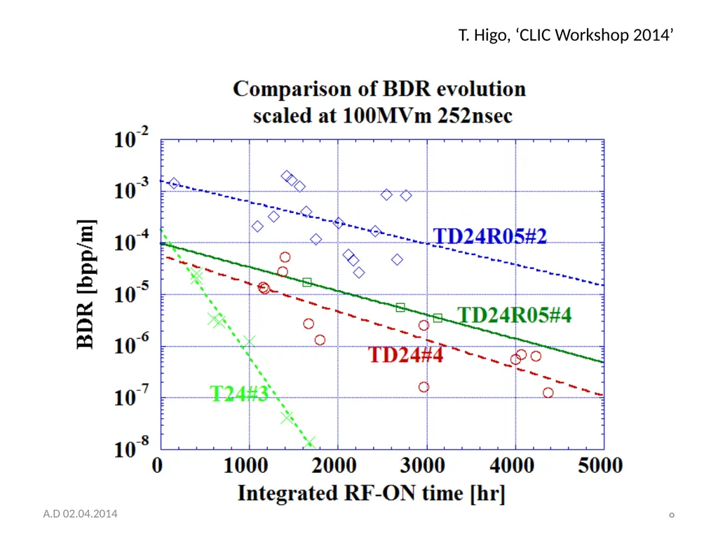
slide7. 7 BDR summary on TD24
comparing to T24 T. Higo, LCWS2012 at Arlington Comparing to T24#3, TD24#4 behaves poor. A.D 02.04.2014<br>
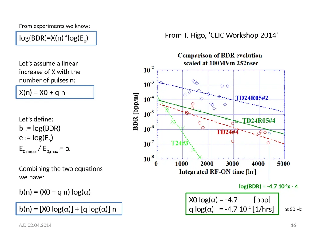
slide8. T. Higo, ‘CLIC Workshop 2014’ A.D 02.04.2014 8<br>
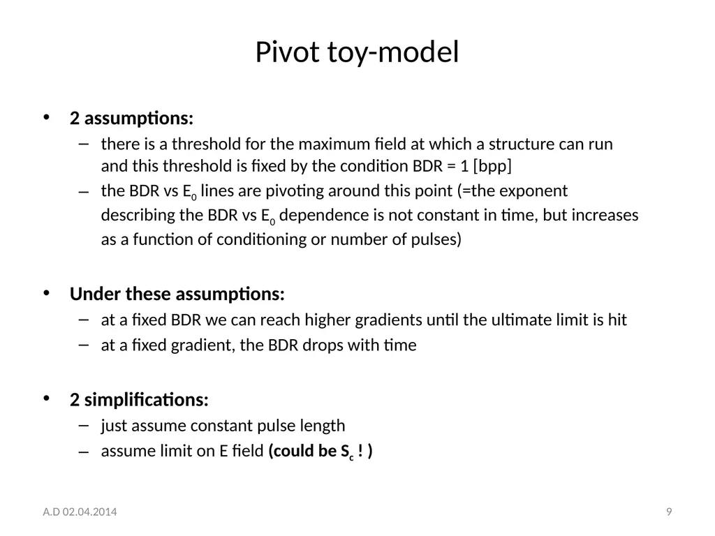
slide9. Pivot toy-model 2 assumptions:
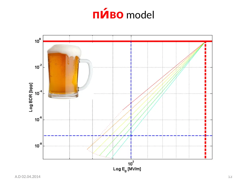
there is a threshold for the maximum field at which a structure can run and this threshold is fixed by the condition BDR = 1 [bpp]
the BDR vs E0 lines are pivoting around this point (=the exponent describing the BDR vs E0 dependence is not constant in time, but increases as a function of conditioning or number of pulses)
Under these assumptions:
at a fixed BDR we can reach higher gradients until the ultimate limit is hit
at a fixed gradient, the BDR drops with time
2 simplifications:
just assume constant pulse length
assume limit on E field (could be Sc ! ) A.D 02.04.2014 9<br>
slide10. Picture of conditioning with pivot model 10 conditioning testing at fixed gradient A.D 02.04.2014<br>
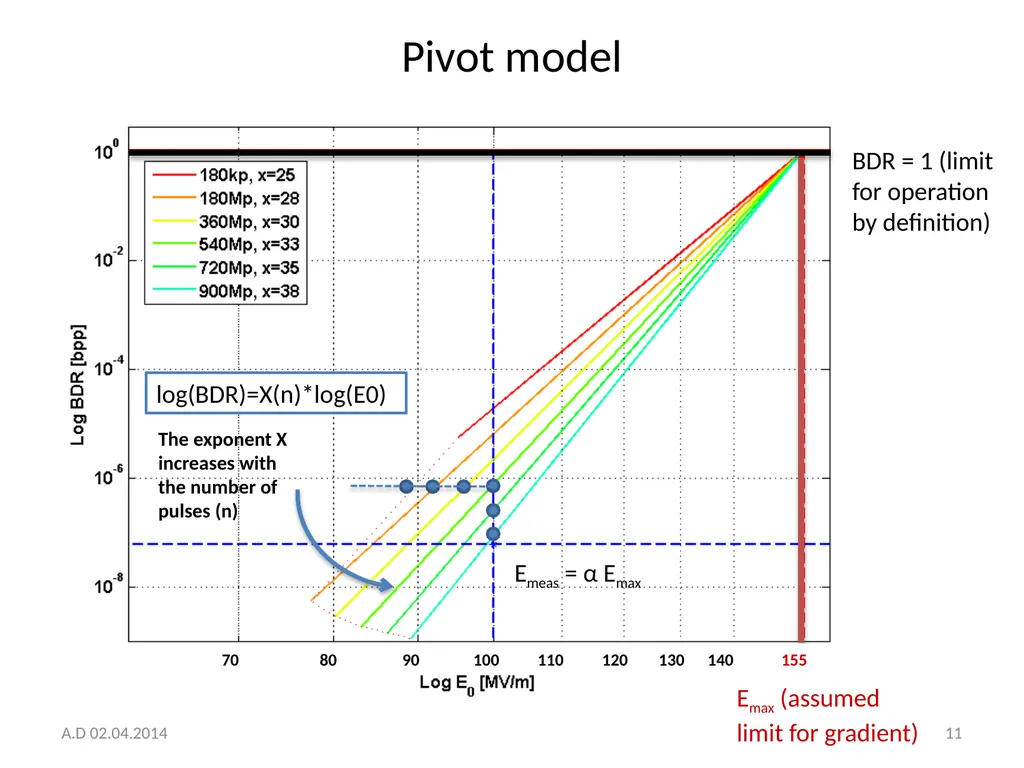
slide11. Pivot model BDR = 1 (limit for operation by definition) Emax (assumed limit for gradient) The exponent X increases with the number of pulses (n) log(BDR)=X(n)*log(E0) Emeas = α Emax 11 70 80 90 100 110 120 130 140 155 A.D 02.04.2014<br>
slide12. Conclusion/discussion and experiment proposal Conditioning strategy
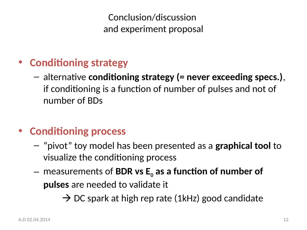
alternative conditioning strategy (= never exceeding specs.), if conditioning is a function of number of pulses and not of number of BDs
Conditioning process
“pivot” toy model has been presented as a graphical tool to visualize the conditioning process
measurements of BDR vs E0 as a function of number of pulses are needed to validate it
DC spark at high rep rate (1kHz) good candidate A.D 02.04.2014 12<br>
slide13. пи́во model 13 A.D 02.04.2014<br>
slide14. thank you for your attention A.D 02.04.2014 14<br>
slide15. extra slides A.D 02.04.2014 15<br>
slide16. log(BDR)=X(n)*log(E0) X(n) = X0 + q n From experiments we know: Let’s define:
b := log(BDR)
e := log(E0)
E0,meas / E0,max = α Let’s assume a linear increase of X with the number of pulses n: b(n) = (X0 + q n) log(α) Combining the two equations we have: b(n) = [X0 log(α)] + [q log(α)] n X0 log(α) = -4.7 [bpp]
q log(α) = -4.7 10-4 [1/hrs] From T. Higo, ‘CLIC Workshop 2014’ log(BDR) = -4.7 10-4x - 4 16 at 50 Hz A.D 02.04.2014<br>
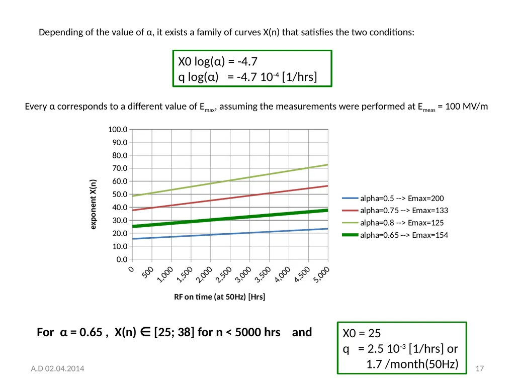
slide17. X0 log(α) = -4.7
q log(α) = -4.7 10-4 [1/hrs] Depending of the value of α, it exists a family of curves X(n) that satisfies the two conditions: Every α corresponds to a different value of Emax, assuming the measurements were performed at Emeas = 100 MV/m For α = 0.65 , X(n) ∈ [25; 38] for n < 5000 hrs and X0 = 25
q = 2.5 10-3 [1/hrs] or
1.7 /month(50Hz) 17 A.D 02.04.2014<br>
slide18. Picture of conditioning 18 conditioning testing at fixed gradient A.D 02.04.2014<br>
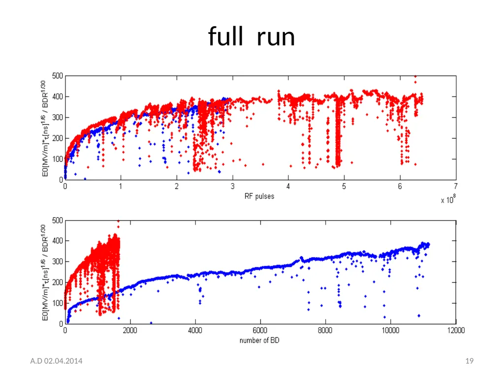
slide19. full run A.D 02.04.2014 19<br>
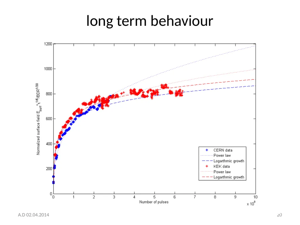
slide20. long term behaviour 20 A.D 02.04.2014<br>
02.04.2014
CLIC RF Structure Development Meeting<br>
slide2. Outline PART 1: conditioning strategy
picture of the current conditioning strategy
proposal of alternative conditioning strategy based on the previous presentation
PART 2: conditioning process
empirical observations
“pivot” toy model A.D 02.04.2014 2<br>
slide3. Picture of the current conditioning strategy 3 1. Conditioning at constant BDR obtained in Xbox1 with long term conditioning algorithm 2. Over shoot and back off to nominal gradient 3. Long term run at 100 MV/m, with typical reduction in BDR A.D 02.04.2014<br>
slide4. Comparison of E0* vs #BD 4 A.D 02.04.2014 Same conditioning level at different number of BD.<br>
slide5. Alternative approach to conditioning: A.D 02.04.2014 5 During conditioning never exceed specs. option 1 option 2<br>
slide6. PART 2: conditioning process Empirical observations about “conditioning”:
during conditioning we can reach higher gradients at a fixed BDR,
at a fixed gradient, the BDR drops with time.
Some questions:
can we go to infinitely high gradients? probably not
can we think to reduce the BDR to extremely low values?
is the dependence between BDR and E0 fixed in time?
What is presented here is a “toy-model”, a graphical way of thinking about how conditioning works, to trigger the discussion A.D 02.04.2014 6<br>
slide7. 7 BDR summary on TD24
comparing to T24 T. Higo, LCWS2012 at Arlington Comparing to T24#3, TD24#4 behaves poor. A.D 02.04.2014<br>
slide8. T. Higo, ‘CLIC Workshop 2014’ A.D 02.04.2014 8<br>
slide9. Pivot toy-model 2 assumptions:
there is a threshold for the maximum field at which a structure can run and this threshold is fixed by the condition BDR = 1 [bpp]
the BDR vs E0 lines are pivoting around this point (=the exponent describing the BDR vs E0 dependence is not constant in time, but increases as a function of conditioning or number of pulses)
Under these assumptions:
at a fixed BDR we can reach higher gradients until the ultimate limit is hit
at a fixed gradient, the BDR drops with time
2 simplifications:
just assume constant pulse length
assume limit on E field (could be Sc ! ) A.D 02.04.2014 9<br>
slide10. Picture of conditioning with pivot model 10 conditioning testing at fixed gradient A.D 02.04.2014<br>
slide11. Pivot model BDR = 1 (limit for operation by definition) Emax (assumed limit for gradient) The exponent X increases with the number of pulses (n) log(BDR)=X(n)*log(E0) Emeas = α Emax 11 70 80 90 100 110 120 130 140 155 A.D 02.04.2014<br>
slide12. Conclusion/discussion and experiment proposal Conditioning strategy
alternative conditioning strategy (= never exceeding specs.), if conditioning is a function of number of pulses and not of number of BDs
Conditioning process
“pivot” toy model has been presented as a graphical tool to visualize the conditioning process
measurements of BDR vs E0 as a function of number of pulses are needed to validate it
DC spark at high rep rate (1kHz) good candidate A.D 02.04.2014 12<br>
slide13. пи́во model 13 A.D 02.04.2014<br>
slide14. thank you for your attention A.D 02.04.2014 14<br>
slide15. extra slides A.D 02.04.2014 15<br>
slide16. log(BDR)=X(n)*log(E0) X(n) = X0 + q n From experiments we know: Let’s define:
b := log(BDR)
e := log(E0)
E0,meas / E0,max = α Let’s assume a linear increase of X with the number of pulses n: b(n) = (X0 + q n) log(α) Combining the two equations we have: b(n) = [X0 log(α)] + [q log(α)] n X0 log(α) = -4.7 [bpp]
q log(α) = -4.7 10-4 [1/hrs] From T. Higo, ‘CLIC Workshop 2014’ log(BDR) = -4.7 10-4x - 4 16 at 50 Hz A.D 02.04.2014<br>
slide17. X0 log(α) = -4.7
q log(α) = -4.7 10-4 [1/hrs] Depending of the value of α, it exists a family of curves X(n) that satisfies the two conditions: Every α corresponds to a different value of Emax, assuming the measurements were performed at Emeas = 100 MV/m For α = 0.65 , X(n) ∈ [25; 38] for n < 5000 hrs and X0 = 25
q = 2.5 10-3 [1/hrs] or
1.7 /month(50Hz) 17 A.D 02.04.2014<br>
slide18. Picture of conditioning 18 conditioning testing at fixed gradient A.D 02.04.2014<br>
slide19. full run A.D 02.04.2014 19<br>
slide20. long term behaviour 20 A.D 02.04.2014<br>