TOPIC IS-LM MODEL YEAR- THIRD SEMESTER-6 SESSION -2022-2023 PAPER NAME MACROECONOMICS II PREPARED BY DR. KAMALIKA CHAKRABORTY ASSISTANT PROFESSOR (DEPARTMENT OF ECONOMICS) KHATRA ADIBASI MAHAVIDYALAYA, BANKURA, WEST BENGAL DATE OF
"TOPIC –IS-LM MODEL YEAR- THIRD SEMESTER-6 SESSION" is the property of its rightful owner. Permission is granted to
download and print the materials on this website for personal, non-commercial use only, and to display it
on your personal computer provided you do not modify the materials and that you retain all copyright
notices contained in the materials. By downloading content from our website, you accept the terms of this
agreement.
Presentation Transcript
01
TOPIC –IS-LM MODEL
YEAR- THIRD SEMESTER-6 SESSION -2022-2023 PAPER NAME – MACROECONOMICS II PREPARED BY
DR. KAMALIKA CHAKRABORTY
ASSISTANT PROFESSOR (DEPARTMENT OF ECONOMICS)
KHATRA ADIBASI MAHAVIDYALAYA, BANKURA, WEST BENGAL DATE OF LECTURE: 4/04/2023 COURSE: B.Sc. (PROGRAMME) IN ECONOMICS<br>
02
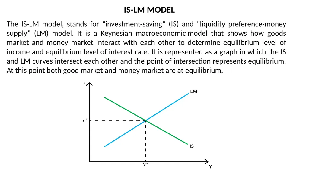
The IS-LM model, stands for “investment-saving” (IS) and “liquidity preference-money supply” (LM) model. It is a Keynesian macroeconomic model that shows how goods market and money market interact with each other to determine equilibrium level of income and equilibrium level of interest rate. It is represented as a graph in which the IS and LM curves intersect each other and the point of intersection represents equilibrium. At this point both good market and money market are at equilibrium. IS-LM MODEL<br>
03
The IS Curve
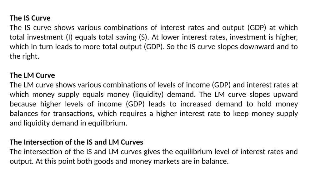
The IS curve shows various combinations of interest rates and output (GDP) at which total investment (I) equals total saving (S). At lower interest rates, investment is higher, which in turn leads to more total output (GDP). So the IS curve slopes downward and to the right.
The LM Curve
The LM curve shows various combinations of levels of income (GDP) and interest rates at which money supply equals money (liquidity) demand. The LM curve slopes upward because higher levels of income (GDP) leads to increased demand to hold money balances for transactions, which requires a higher interest rate to keep money supply and liquidity demand in equilibrium.
The Intersection of the IS and LM Curves
The intersection of the IS and LM curves gives the equilibrium level of interest rates and output. At this point both goods and money markets are in balance.<br>
04
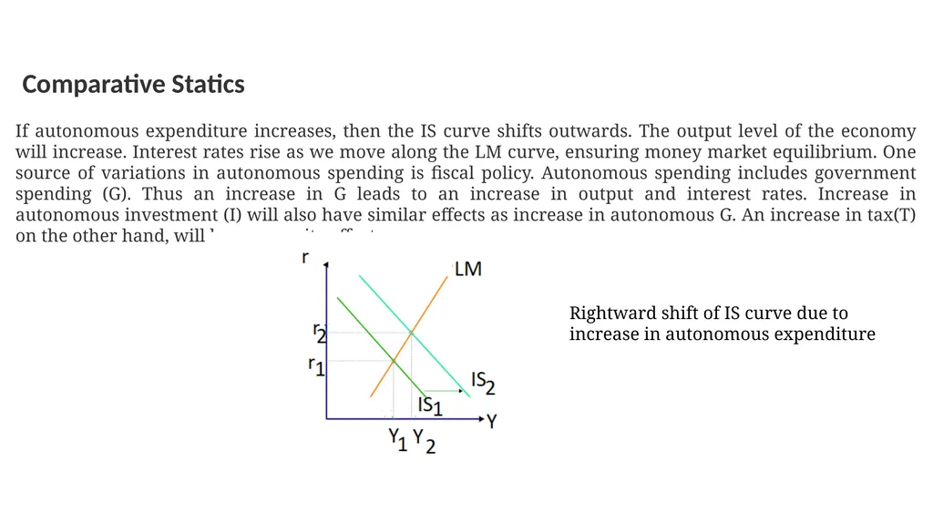
Comparative Statics If autonomous expenditure increases, then the IS curve shifts outwards. The output level of the economy will increase. Interest rates rise as we move along the LM curve, ensuring money market equilibrium. One source of variations in autonomous spending is fiscal policy. Autonomous spending includes government spending (G). Thus an increase in G leads to an increase in output and interest rates. Increase in autonomous investment (I) will also have similar effects as increase in autonomous G. An increase in tax(T) on the other hand, will have opposite effects. Rightward shift of IS curve due to increase in autonomous expenditure<br>
05
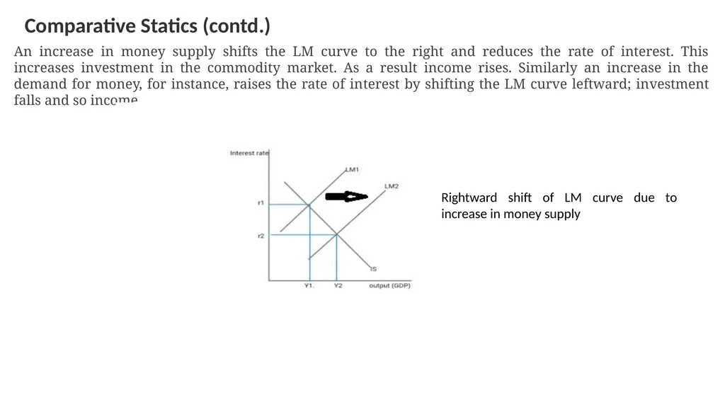
Comparative Statics (contd.) An increase in money supply shifts the LM curve to the right and reduces the rate of interest. This increases investment in the commodity market. As a result income rises. Similarly an increase in the demand for money, for instance, raises the rate of interest by shifting the LM curve leftward; investment falls and so income. Rightward shift of LM curve due to increase in money supply<br>