
Various Options in Building Neural Networks:
PM
Published · 56 slides · 0 views

1 / 1


Description
Various Options in Building Neural Networks: Activation Functions, Loss Functions, Optimizers, Batch Size, Dropout CSE 4311 Neural Networks and Deep Learning Vassilis Athitsos Computer Science and Engineering Department University of
Related Topics
Share
Embed code
Download this presentation From Below
"Various Options in Building Neural Networks:" is the property of its rightful owner. Permission is granted to download and print the materials on this website for personal, non-commercial use only, and to display it on your personal computer provided you do not modify the materials and that you retain all copyright notices contained in the materials. By downloading content from our website, you accept the terms of this agreement.
Presentation Transcript
01
Various Options in Building Neural Networks:
Activation Functions, Loss Functions, Optimizers, Batch Size, Dropout CSE 4311 – Neural Networks and Deep Learning
Vassilis Athitsos
Computer Science and Engineering Department
University of Texas at Arlington 1<br>
Vassilis Athitsos
Computer Science and Engineering Department
University of Texas at Arlington 1<br>
02
Expanding our Options So far, we focused on training and testing a complete neural network.
To keep things simple, we did not explore many options.
Here is what we have tried so far:
Activation function: sigmoid
Layer type: fully connected (called “dense” in Keras).
Loss function: SSD in homework 3, CCE in Keras example (but we have not defined CCE yet).
Optimization: ad hoc method in homework 3, “Adam” in Keras example (but we have not defined “Adam” yet).
Now it is time to get familiar with more options, so that we can start using them.
Different choices are best for different situations, it is good to experiment with different options. 2<br>
To keep things simple, we did not explore many options.
Here is what we have tried so far:
Activation function: sigmoid
Layer type: fully connected (called “dense” in Keras).
Loss function: SSD in homework 3, CCE in Keras example (but we have not defined CCE yet).
Optimization: ad hoc method in homework 3, “Adam” in Keras example (but we have not defined “Adam” yet).
Now it is time to get familiar with more options, so that we can start using them.
Different choices are best for different situations, it is good to experiment with different options. 2<br>
03
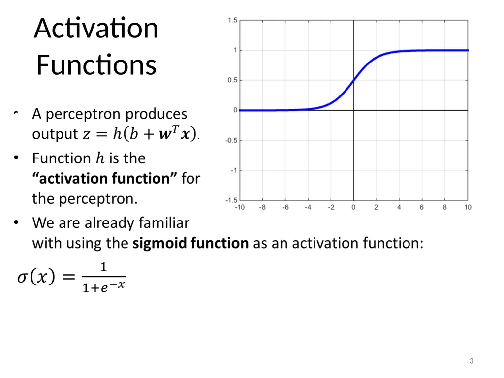
Activation Functions 3<br>
04
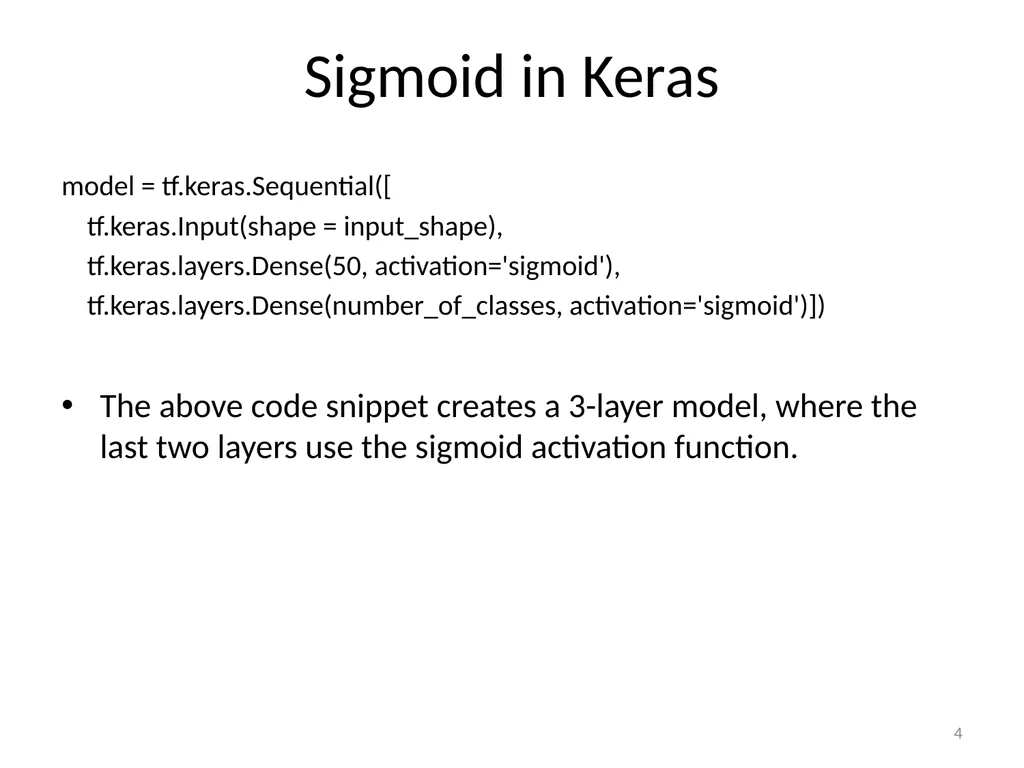
Sigmoid in Keras model = tf.keras.Sequential([
tf.keras.Input(shape = input_shape),
tf.keras.layers.Dense(50, activation='sigmoid'),
tf.keras.layers.Dense(number_of_classes, activation='sigmoid')])
The above code snippet creates a 3-layer model, where the last two layers use the sigmoid activation function. 4<br>
tf.keras.Input(shape = input_shape),
tf.keras.layers.Dense(50, activation='sigmoid'),
tf.keras.layers.Dense(number_of_classes, activation='sigmoid')])
The above code snippet creates a 3-layer model, where the last two layers use the sigmoid activation function. 4<br>
05
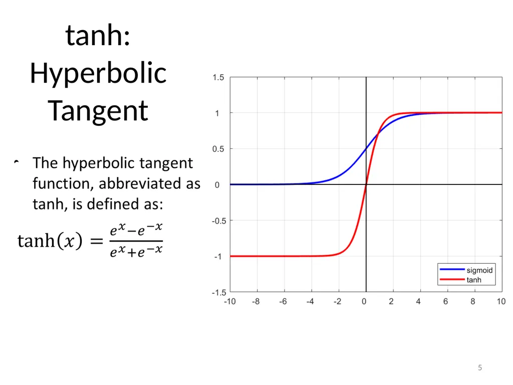
tanh: Hyperbolic Tangent 5<br>
06
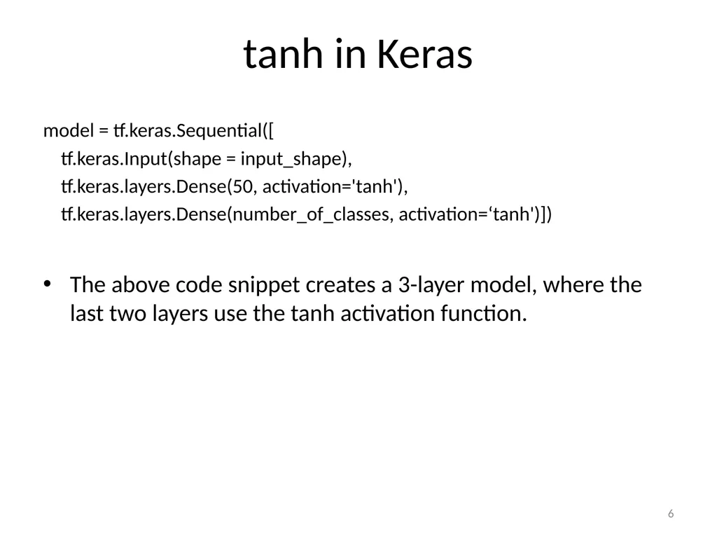
tanh in Keras model = tf.keras.Sequential([
tf.keras.Input(shape = input_shape),
tf.keras.layers.Dense(50, activation='tanh'),
tf.keras.layers.Dense(number_of_classes, activation=‘tanh')])
The above code snippet creates a 3-layer model, where the last two layers use the tanh activation function. 6<br>
tf.keras.Input(shape = input_shape),
tf.keras.layers.Dense(50, activation='tanh'),
tf.keras.layers.Dense(number_of_classes, activation=‘tanh')])
The above code snippet creates a 3-layer model, where the last two layers use the tanh activation function. 6<br>
07
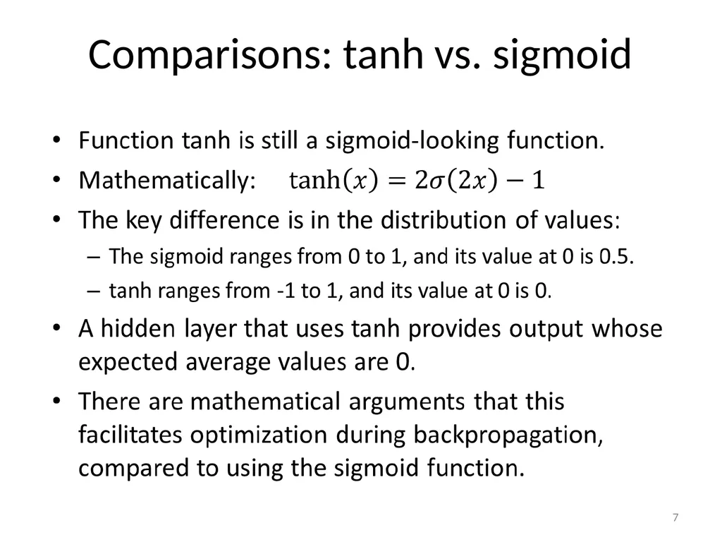
Comparisons: tanh vs. sigmoid 7<br>
08
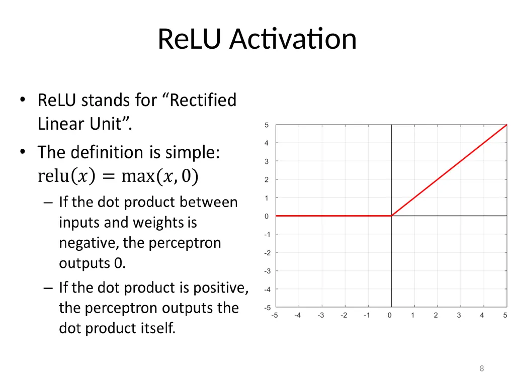
ReLU Activation 8<br>
09
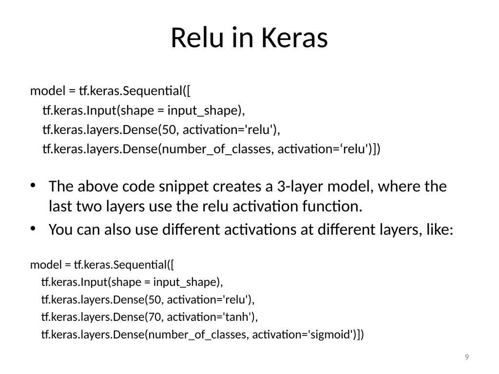
Relu in Keras model = tf.keras.Sequential([
tf.keras.Input(shape = input_shape),
tf.keras.layers.Dense(50, activation='relu'),
tf.keras.layers.Dense(number_of_classes, activation=‘relu')])
The above code snippet creates a 3-layer model, where the last two layers use the relu activation function.
You can also use different activations at different layers, like:
model = tf.keras.Sequential([
tf.keras.Input(shape = input_shape),
tf.keras.layers.Dense(50, activation='relu'),
tf.keras.layers.Dense(70, activation='tanh'),
tf.keras.layers.Dense(number_of_classes, activation='sigmoid')]) 9<br>
tf.keras.Input(shape = input_shape),
tf.keras.layers.Dense(50, activation='relu'),
tf.keras.layers.Dense(number_of_classes, activation=‘relu')])
The above code snippet creates a 3-layer model, where the last two layers use the relu activation function.
You can also use different activations at different layers, like:
model = tf.keras.Sequential([
tf.keras.Input(shape = input_shape),
tf.keras.layers.Dense(50, activation='relu'),
tf.keras.layers.Dense(70, activation='tanh'),
tf.keras.layers.Dense(number_of_classes, activation='sigmoid')]) 9<br>
10
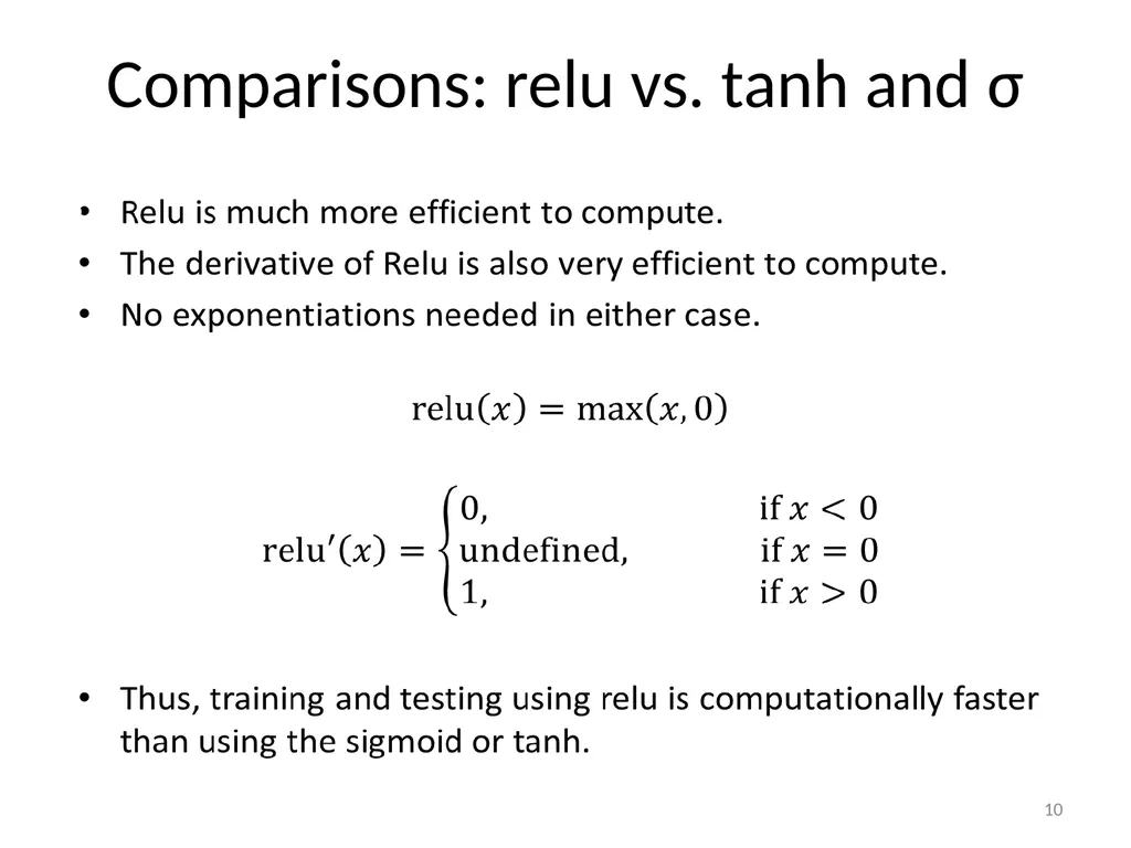
Comparisons: relu vs. tanh and σ 10<br>
11
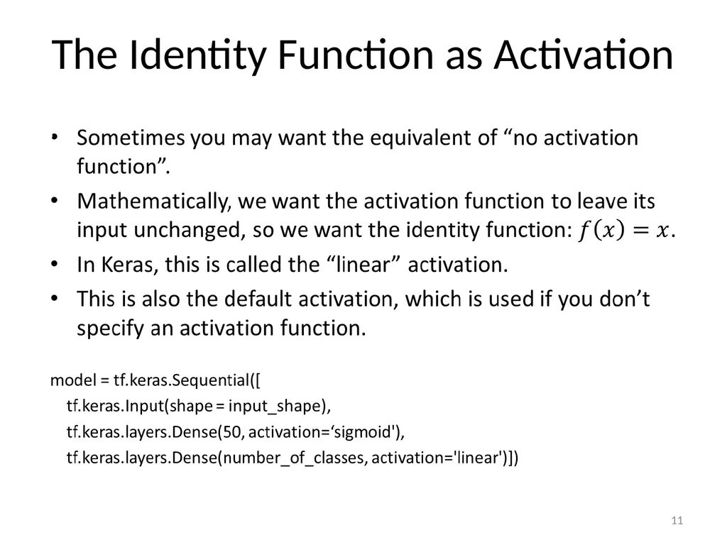
The Identity Function as Activation 11<br>
12
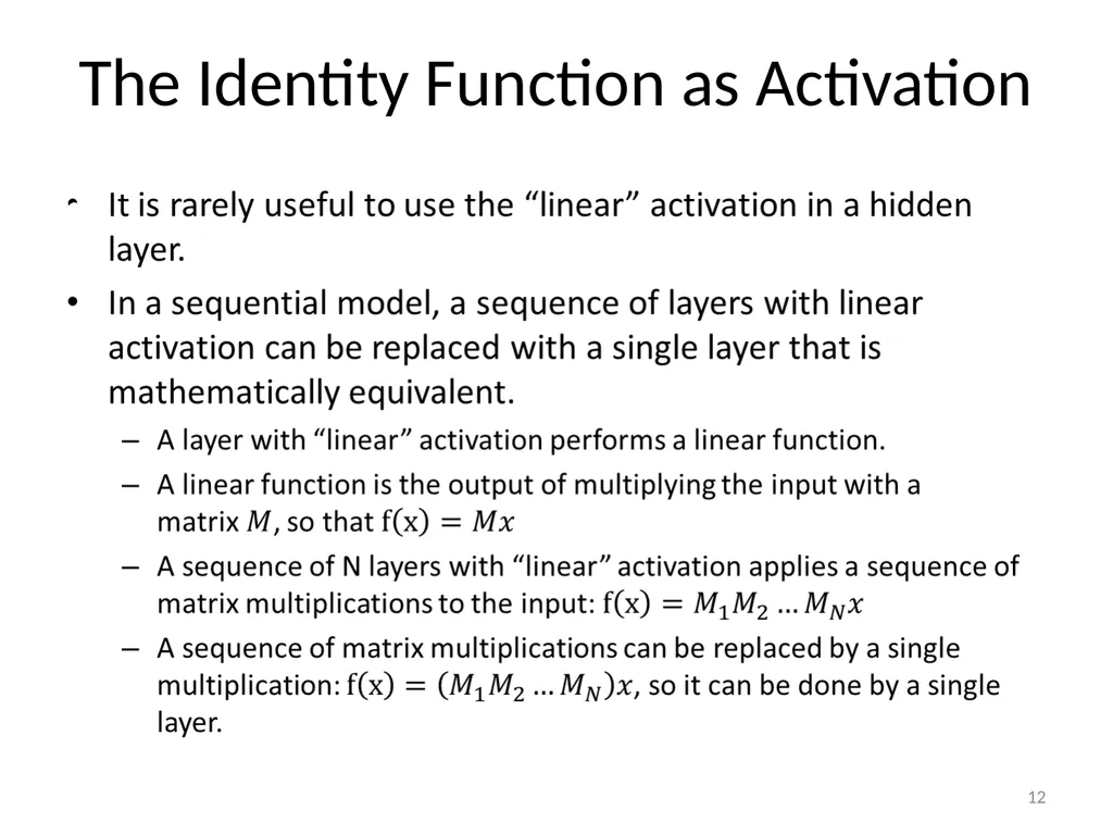
The Identity Function as Activation 12<br>
13
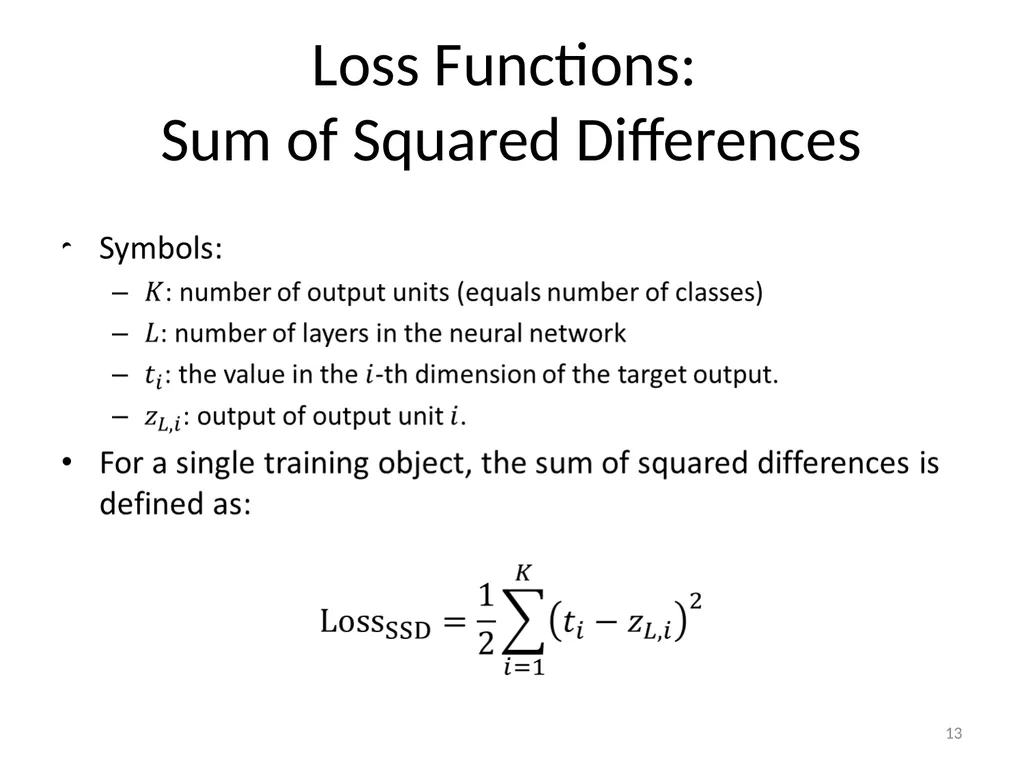
Loss Functions:
Sum of Squared Differences 13<br>
14
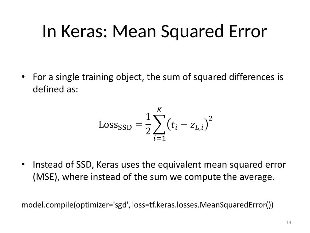
In Keras: Mean Squared Error 14<br>
15
Loss Functions:
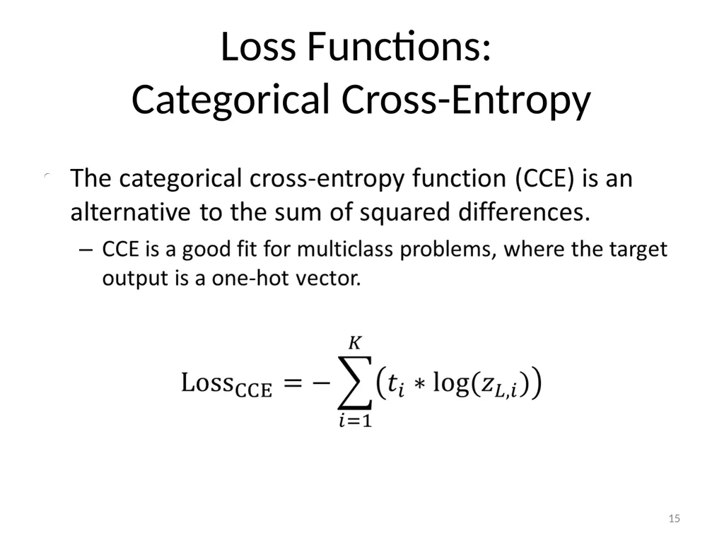
Categorical Cross-Entropy 15<br>
16
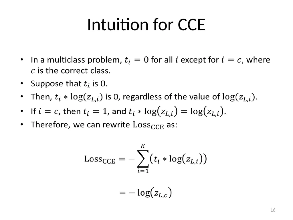
Intuition for CCE 16<br>
17
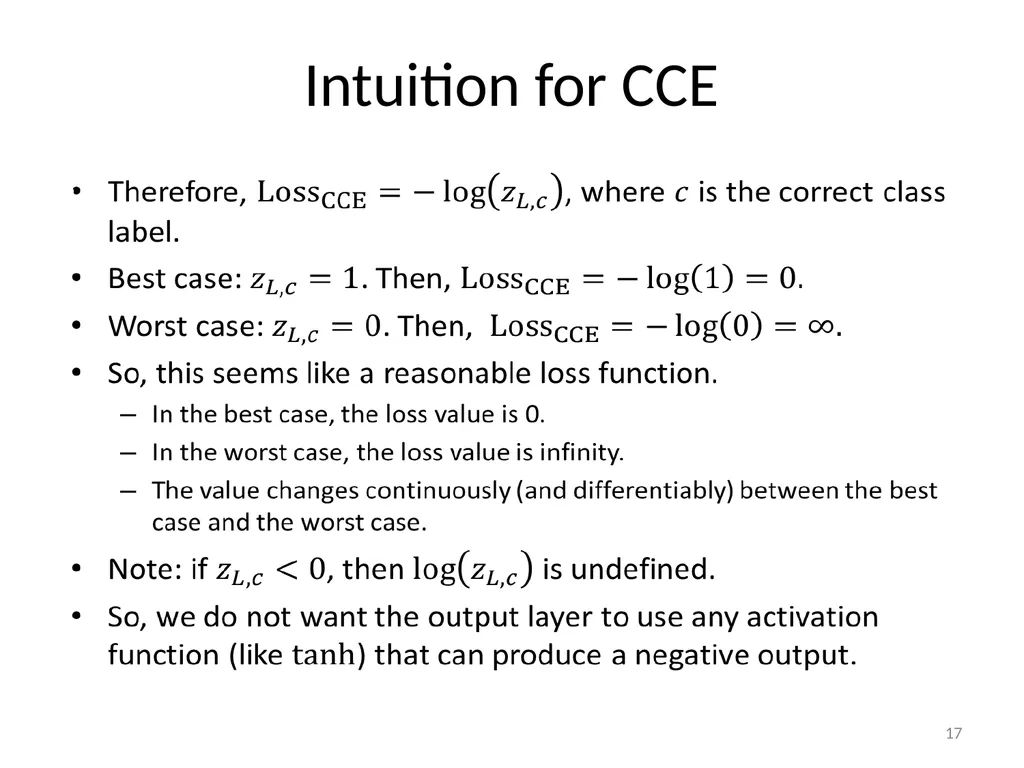
Intuition for CCE 17<br>
18
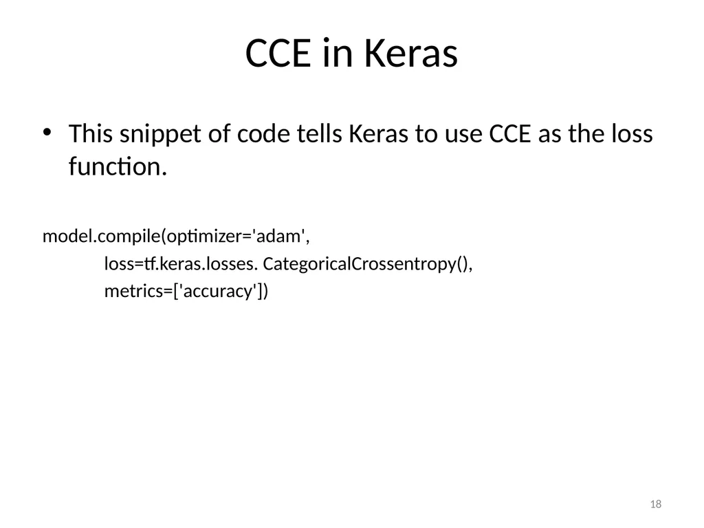
CCE in Keras This snippet of code tells Keras to use CCE as the loss function.
model.compile(optimizer='adam',
loss=tf.keras.losses. CategoricalCrossentropy(),
metrics=['accuracy']) 18<br>
model.compile(optimizer='adam',
loss=tf.keras.losses. CategoricalCrossentropy(),
metrics=['accuracy']) 18<br>
19
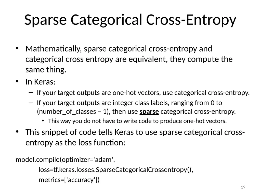
Sparse Categorical Cross-Entropy Mathematically, sparse categorical cross-entropy and categorical cross entropy are equivalent, they compute the same thing.
In Keras:
If your target outputs are one-hot vectors, use categorical cross-entropy.
If your target outputs are integer class labels, ranging from 0 to (number_of_classes – 1), then use sparse categorical cross-entropy.
This way you do not have to write code to produce one-hot vectors.
This snippet of code tells Keras to use sparse categorical cross-entropy as the loss function:
model.compile(optimizer='adam',
loss=tf.keras.losses.SparseCategoricalCrossentropy(),
metrics=['accuracy']) 19<br>
In Keras:
If your target outputs are one-hot vectors, use categorical cross-entropy.
If your target outputs are integer class labels, ranging from 0 to (number_of_classes – 1), then use sparse categorical cross-entropy.
This way you do not have to write code to produce one-hot vectors.
This snippet of code tells Keras to use sparse categorical cross-entropy as the loss function:
model.compile(optimizer='adam',
loss=tf.keras.losses.SparseCategoricalCrossentropy(),
metrics=['accuracy']) 19<br>
20
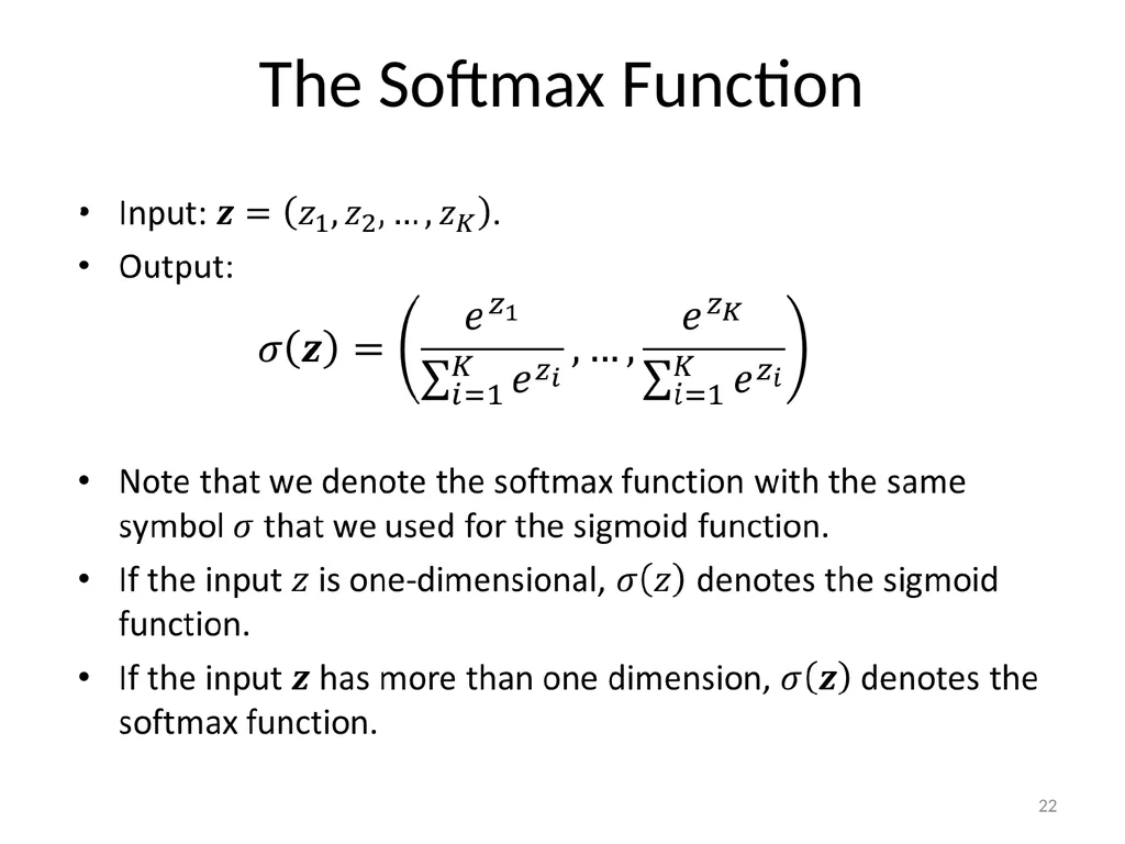
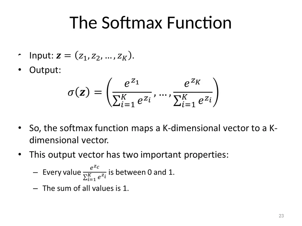
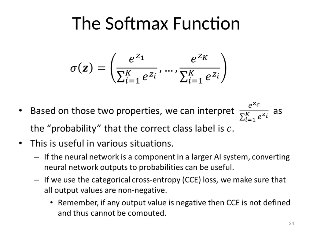
The Softmax Function When we train a neural network for multiclass classification, it is very common to use a “softmax output layer”.
Typically, “softmax output layers” go hand-in-hand with the categorical cross-entropy loss function.
The reason for the quotes in “softmax layer” is that it does not match our current definition of what a “layer” is.
To add to the confusion, sometimes people use the term “softmax layer”, sometimes they use the term “softmax activation function”.
We will have the same problem with other commonly used “layers”.
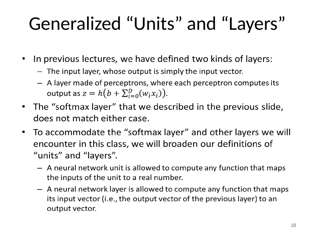
To address that, we will expand our definition of what a “unit” is and what a “layer” is. 20<br>
Typically, “softmax output layers” go hand-in-hand with the categorical cross-entropy loss function.
The reason for the quotes in “softmax layer” is that it does not match our current definition of what a “layer” is.
To add to the confusion, sometimes people use the term “softmax layer”, sometimes they use the term “softmax activation function”.
We will have the same problem with other commonly used “layers”.
To address that, we will expand our definition of what a “unit” is and what a “layer” is. 20<br>
21
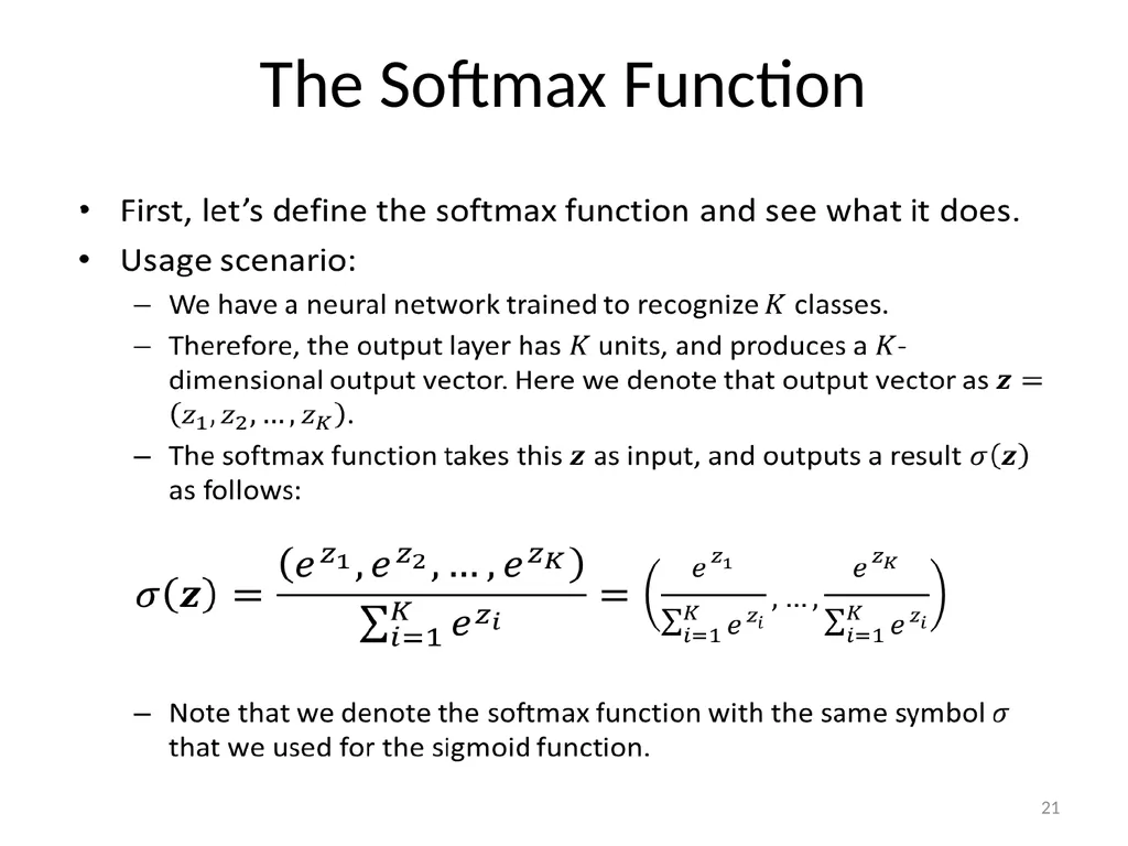
The Softmax Function 21<br>
22
The Softmax Function 22<br>
23
The Softmax Function 23<br>
24
The Softmax Function 24<br>
25
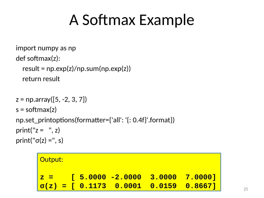
A Softmax Example import numpy as np
def softmax(z):
result = np.exp(z)/np.sum(np.exp(z))
return result
z = np.array([5, -2, 3, 7])
s = softmax(z)
np.set_printoptions(formatter={'all': '{: 0.4f}'.format})
print("z = ", z)
print("σ(z) =", s) 25 Output:
z = [ 5.0000 -2.0000 3.0000 7.0000]
σ(z) = [ 0.1173 0.0001 0.0159 0.8667]<br>
def softmax(z):
result = np.exp(z)/np.sum(np.exp(z))
return result
z = np.array([5, -2, 3, 7])
s = softmax(z)
np.set_printoptions(formatter={'all': '{: 0.4f}'.format})
print("z = ", z)
print("σ(z) =", s) 25 Output:
z = [ 5.0000 -2.0000 3.0000 7.0000]
σ(z) = [ 0.1173 0.0001 0.0159 0.8667]<br>
26
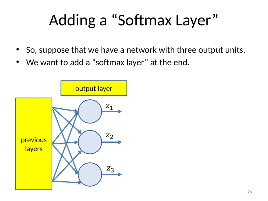
Adding a “Softmax Layer” So, suppose that we have a network with three output units.
We want to add a “softmax layer” at the end. 26 26 previous layers output layer<br>
We want to add a “softmax layer” at the end. 26 26 previous layers output layer<br>
27
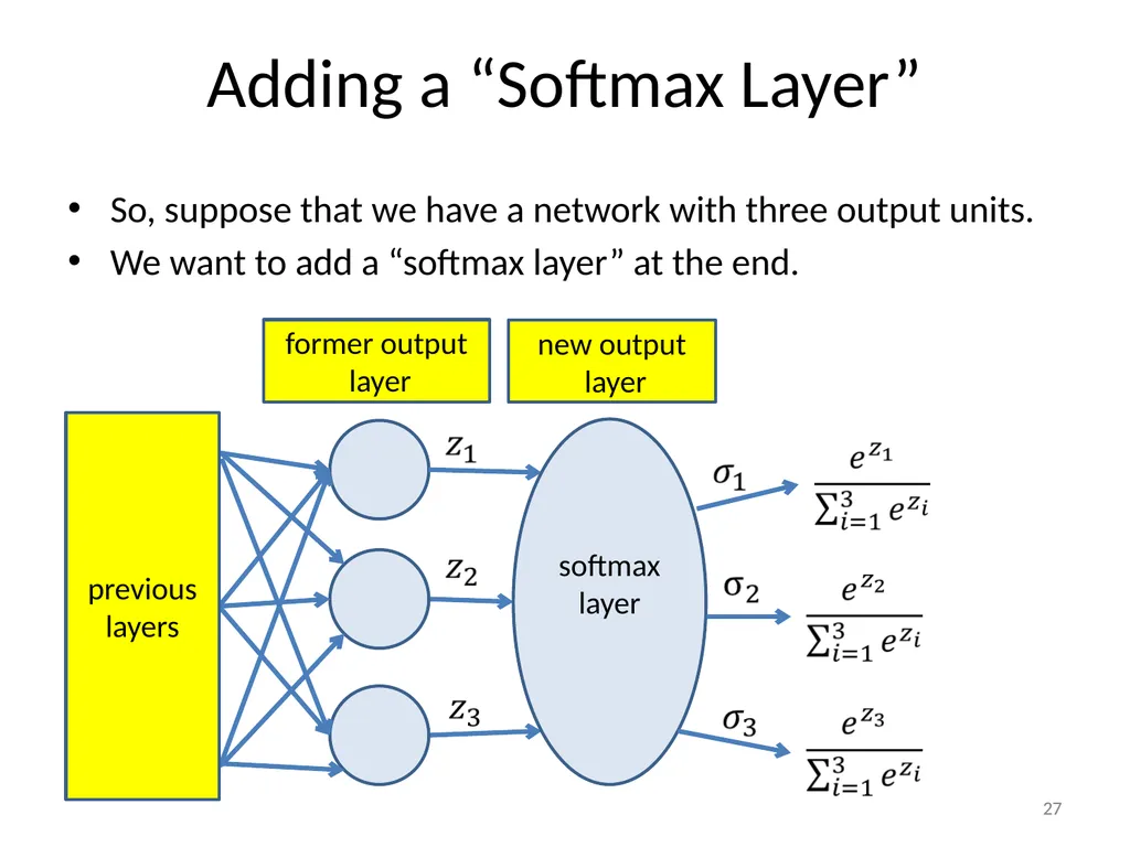
Adding a “Softmax Layer” So, suppose that we have a network with three output units.
We want to add a “softmax layer” at the end. 27 27 previous layers former output layer softmax layer new output layer<br>
We want to add a “softmax layer” at the end. 27 27 previous layers former output layer softmax layer new output layer<br>
28
Generalized “Units” and “Layers” 28 28<br>
29
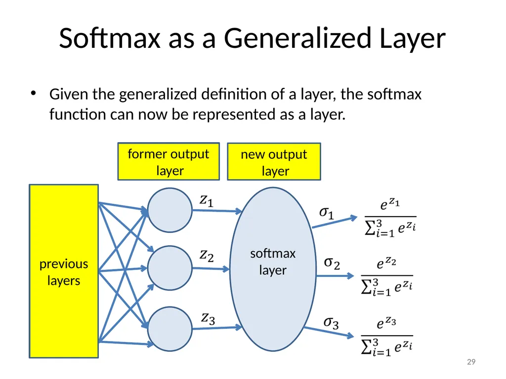
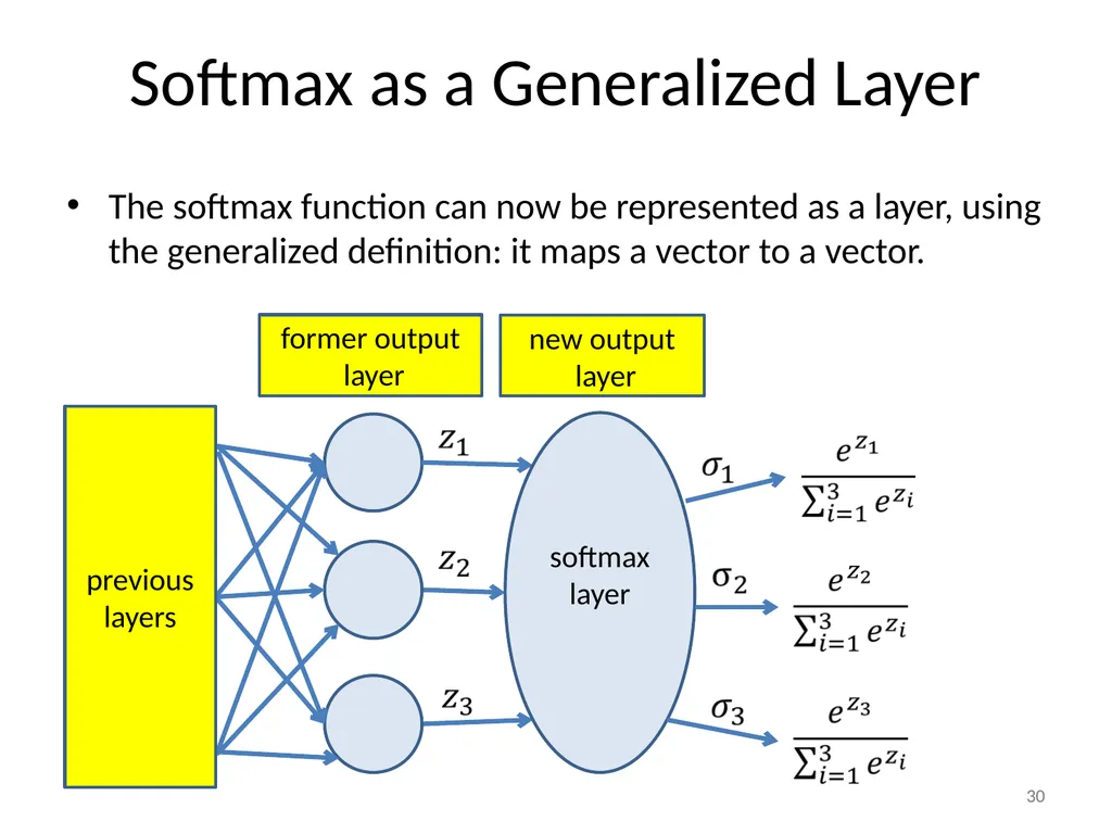
Softmax as a Generalized Layer Given the generalized definition of a layer, the softmax function can now be represented as a layer. 29 29 previous layers former output
layer softmax
layer new output
layer<br>
30
Softmax as a Generalized Layer The softmax function can now be represented as a layer, using the generalized definition: it maps a vector to a vector. 30 30 previous layers former output
layer softmax
layer new output
layer<br>
31
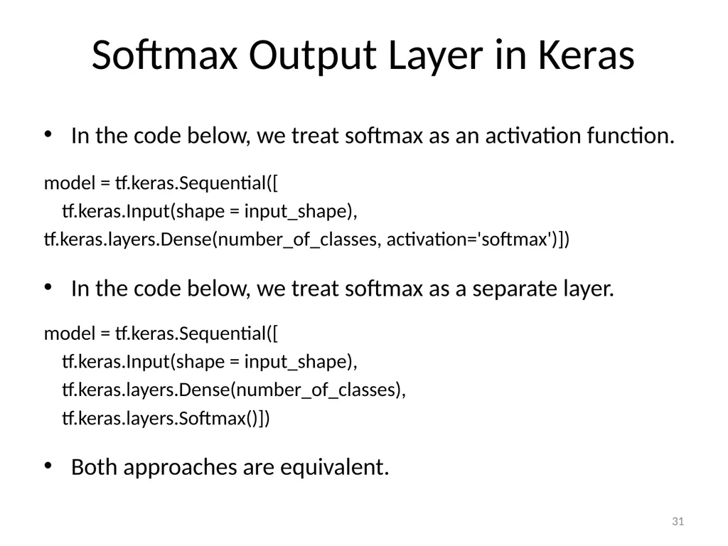
Softmax Output Layer in Keras In the code below, we treat softmax as an activation function.
model = tf.keras.Sequential([
tf.keras.Input(shape = input_shape),
tf.keras.layers.Dense(number_of_classes, activation='softmax')])
In the code below, we treat softmax as a separate layer.
model = tf.keras.Sequential([
tf.keras.Input(shape = input_shape),
tf.keras.layers.Dense(number_of_classes),
tf.keras.layers.Softmax()])
Both approaches are equivalent. 31<br>
model = tf.keras.Sequential([
tf.keras.Input(shape = input_shape),
tf.keras.layers.Dense(number_of_classes, activation='softmax')])
In the code below, we treat softmax as a separate layer.
model = tf.keras.Sequential([
tf.keras.Input(shape = input_shape),
tf.keras.layers.Dense(number_of_classes),
tf.keras.layers.Softmax()])
Both approaches are equivalent. 31<br>
32
import tensorflow as tf
import numpy as np
from uci_data import *
# loading the dataset
(training_set, test_set) = read_uci1("uci_datasets", "pendigits")
(training_inputs, training_labels) = training_set
(test_inputs, test_labels) = test_set
max_value = np.max(np.abs(training_inputs))
training_inputs = training_inputs / max_value
test_inputs = test_inputs/ max_value
# Creating the model
input_shape = training_inputs[0].shape
number_of_classes = np.max([np.max(training_labels), np.max(test_labels)]) + 1
model = tf.keras.Sequential([
tf.keras.Input(shape = input_shape),
tf.keras.layers.Dense(70, activation='tanh'),
tf.keras.layers.Dense(number_of_classes, activation='softmax')])
model.compile(optimizer='adam', loss=tf.keras.losses.SparseCategoricalCrossentropy(), metrics=['accuracy'])
# Training the model
model.fit(training_inputs, training_labels, epochs=10)
# Testing the model
test_loss, test_acc = model.evaluate(test_inputs, test_labels, verbose=0)
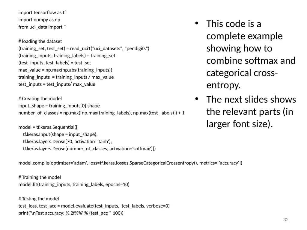
print('\nTest accuracy: %.2f%%' % (test_acc * 100)) 32 This code is a complete example showing how to combine softmax and categorical cross-entropy.
The next slides shows the relevant parts (in larger font size).<br>
import numpy as np
from uci_data import *
# loading the dataset
(training_set, test_set) = read_uci1("uci_datasets", "pendigits")
(training_inputs, training_labels) = training_set
(test_inputs, test_labels) = test_set
max_value = np.max(np.abs(training_inputs))
training_inputs = training_inputs / max_value
test_inputs = test_inputs/ max_value
# Creating the model
input_shape = training_inputs[0].shape
number_of_classes = np.max([np.max(training_labels), np.max(test_labels)]) + 1
model = tf.keras.Sequential([
tf.keras.Input(shape = input_shape),
tf.keras.layers.Dense(70, activation='tanh'),
tf.keras.layers.Dense(number_of_classes, activation='softmax')])
model.compile(optimizer='adam', loss=tf.keras.losses.SparseCategoricalCrossentropy(), metrics=['accuracy'])
# Training the model
model.fit(training_inputs, training_labels, epochs=10)
# Testing the model
test_loss, test_acc = model.evaluate(test_inputs, test_labels, verbose=0)
print('\nTest accuracy: %.2f%%' % (test_acc * 100)) 32 This code is a complete example showing how to combine softmax and categorical cross-entropy.
The next slides shows the relevant parts (in larger font size).<br>
33
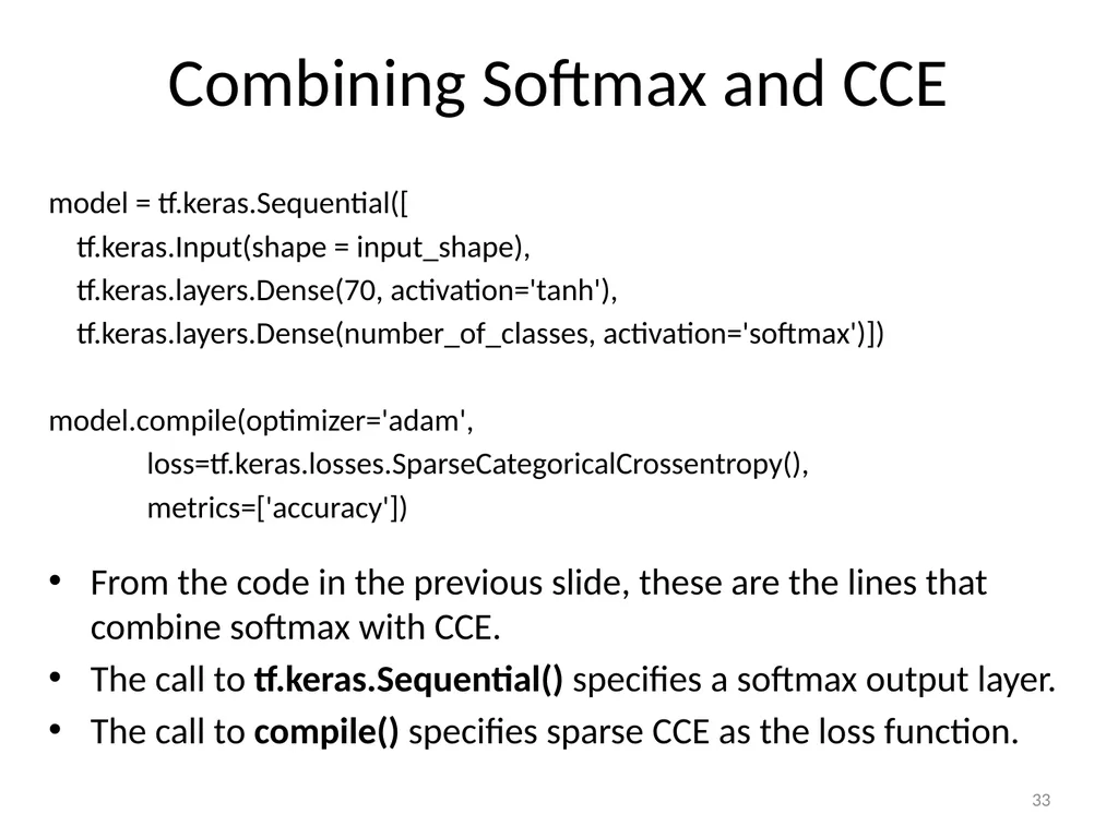
Combining Softmax and CCE model = tf.keras.Sequential([
tf.keras.Input(shape = input_shape),
tf.keras.layers.Dense(70, activation='tanh'),
tf.keras.layers.Dense(number_of_classes, activation='softmax')])
model.compile(optimizer='adam',
loss=tf.keras.losses.SparseCategoricalCrossentropy(),
metrics=['accuracy'])
From the code in the previous slide, these are the lines that combine softmax with CCE.
The call to tf.keras.Sequential() specifies a softmax output layer.
The call to compile() specifies sparse CCE as the loss function. 33<br>
tf.keras.Input(shape = input_shape),
tf.keras.layers.Dense(70, activation='tanh'),
tf.keras.layers.Dense(number_of_classes, activation='softmax')])
model.compile(optimizer='adam',
loss=tf.keras.losses.SparseCategoricalCrossentropy(),
metrics=['accuracy'])
From the code in the previous slide, these are the lines that combine softmax with CCE.
The call to tf.keras.Sequential() specifies a softmax output layer.
The call to compile() specifies sparse CCE as the loss function. 33<br>
34
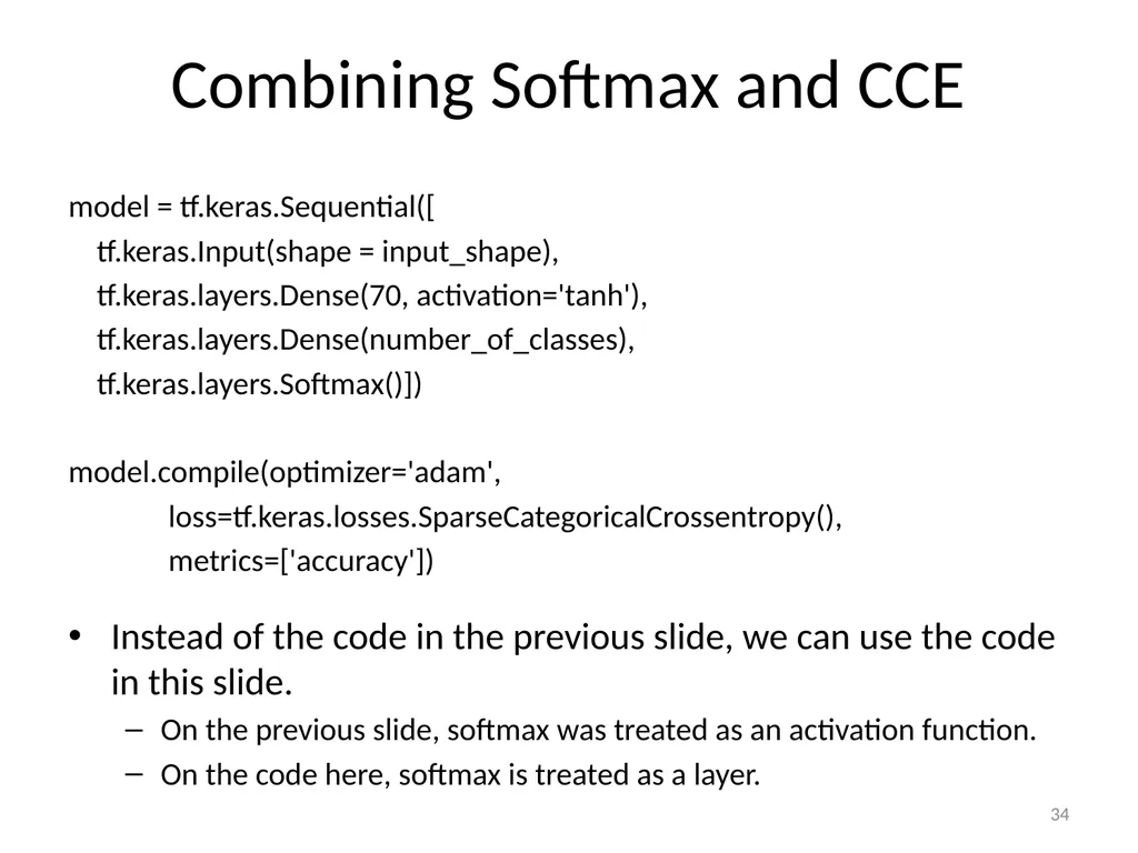
Combining Softmax and CCE model = tf.keras.Sequential([
tf.keras.Input(shape = input_shape),
tf.keras.layers.Dense(70, activation='tanh'),
tf.keras.layers.Dense(number_of_classes),
tf.keras.layers.Softmax()])
model.compile(optimizer='adam',
loss=tf.keras.losses.SparseCategoricalCrossentropy(),
metrics=['accuracy'])
Instead of the code in the previous slide, we can use the code in this slide.
On the previous slide, softmax was treated as an activation function.
On the code here, softmax is treated as a layer. 34<br>
tf.keras.Input(shape = input_shape),
tf.keras.layers.Dense(70, activation='tanh'),
tf.keras.layers.Dense(number_of_classes),
tf.keras.layers.Softmax()])
model.compile(optimizer='adam',
loss=tf.keras.losses.SparseCategoricalCrossentropy(),
metrics=['accuracy'])
Instead of the code in the previous slide, we can use the code in this slide.
On the previous slide, softmax was treated as an activation function.
On the code here, softmax is treated as a layer. 34<br>
35
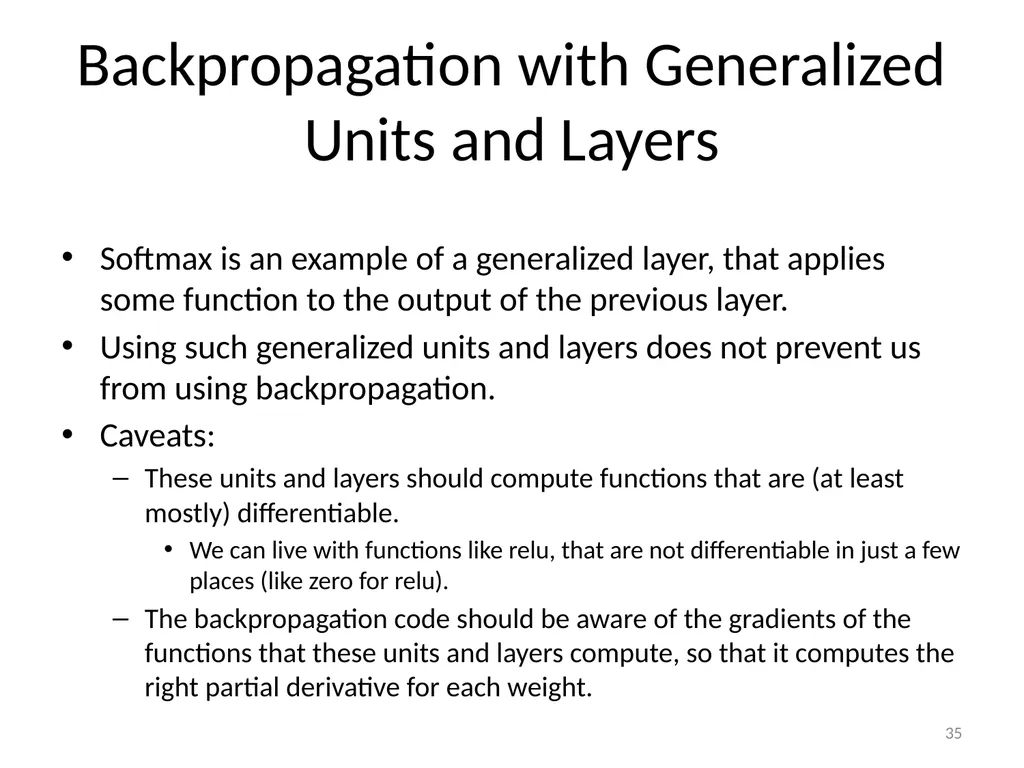
Backpropagation with Generalized Units and Layers Softmax is an example of a generalized layer, that applies some function to the output of the previous layer.
Using such generalized units and layers does not prevent us from using backpropagation.
Caveats:
These units and layers should compute functions that are (at least mostly) differentiable.
We can live with functions like relu, that are not differentiable in just a few places (like zero for relu).
The backpropagation code should be aware of the gradients of the functions that these units and layers compute, so that it computes the right partial derivative for each weight. 35<br>
Using such generalized units and layers does not prevent us from using backpropagation.
Caveats:
These units and layers should compute functions that are (at least mostly) differentiable.
We can live with functions like relu, that are not differentiable in just a few places (like zero for relu).
The backpropagation code should be aware of the gradients of the functions that these units and layers compute, so that it computes the right partial derivative for each weight. 35<br>
36
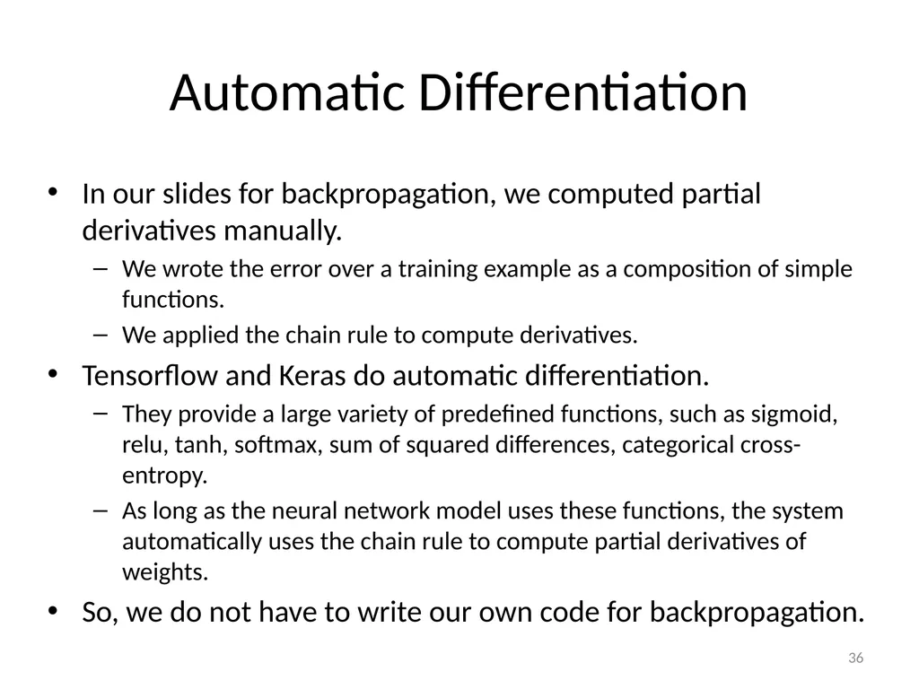
Automatic Differentiation In our slides for backpropagation, we computed partial derivatives manually.
We wrote the error over a training example as a composition of simple functions.
We applied the chain rule to compute derivatives.
Tensorflow and Keras do automatic differentiation.
They provide a large variety of predefined functions, such as sigmoid, relu, tanh, softmax, sum of squared differences, categorical cross-entropy.
As long as the neural network model uses these functions, the system automatically uses the chain rule to compute partial derivatives of weights.
So, we do not have to write our own code for backpropagation. 36<br>
We wrote the error over a training example as a composition of simple functions.
We applied the chain rule to compute derivatives.
Tensorflow and Keras do automatic differentiation.
They provide a large variety of predefined functions, such as sigmoid, relu, tanh, softmax, sum of squared differences, categorical cross-entropy.
As long as the neural network model uses these functions, the system automatically uses the chain rule to compute partial derivatives of weights.
So, we do not have to write our own code for backpropagation. 36<br>
37
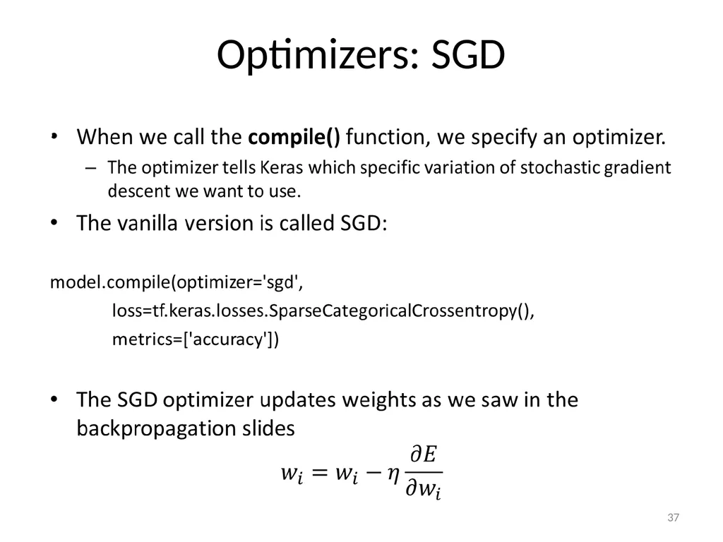
Optimizers: SGD 37<br>
38
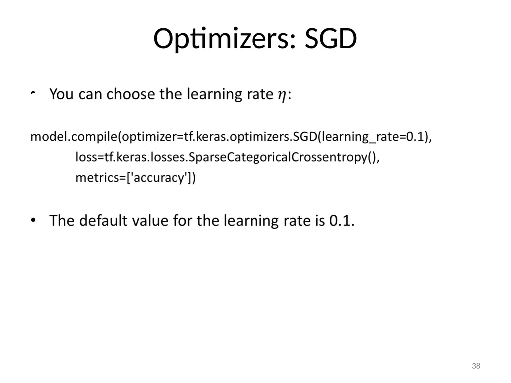
Optimizers: SGD 38<br>
39
Optimizers: SGD with Momentum 39<br>
40
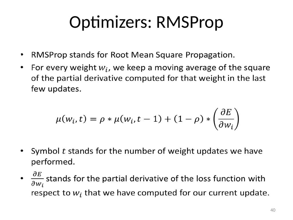
Optimizers: RMSProp 40<br>
41
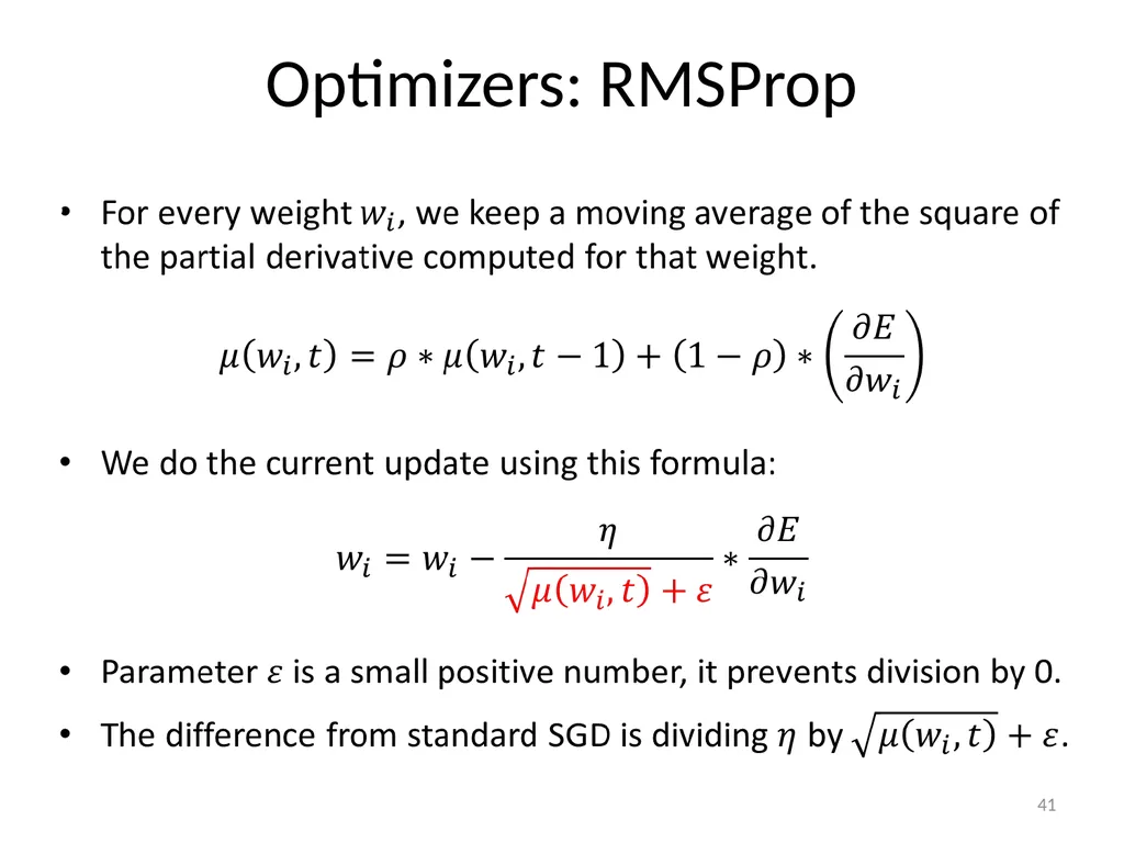
Optimizers: RMSProp 41<br>
42
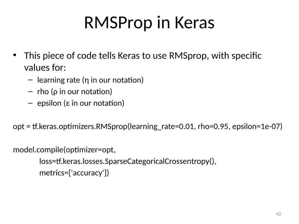
RMSProp in Keras This piece of code tells Keras to use RMSprop, with specific values for:
learning rate (η in our notation)
rho (ρ in our notation)
epsilon (ε in our notation)
opt = tf.keras.optimizers.RMSprop(learning_rate=0.01, rho=0.95, epsilon=1e-07)
model.compile(optimizer=opt,
loss=tf.keras.losses.SparseCategoricalCrossentropy(),
metrics=['accuracy']) 42<br>
learning rate (η in our notation)
rho (ρ in our notation)
epsilon (ε in our notation)
opt = tf.keras.optimizers.RMSprop(learning_rate=0.01, rho=0.95, epsilon=1e-07)
model.compile(optimizer=opt,
loss=tf.keras.losses.SparseCategoricalCrossentropy(),
metrics=['accuracy']) 42<br>
43
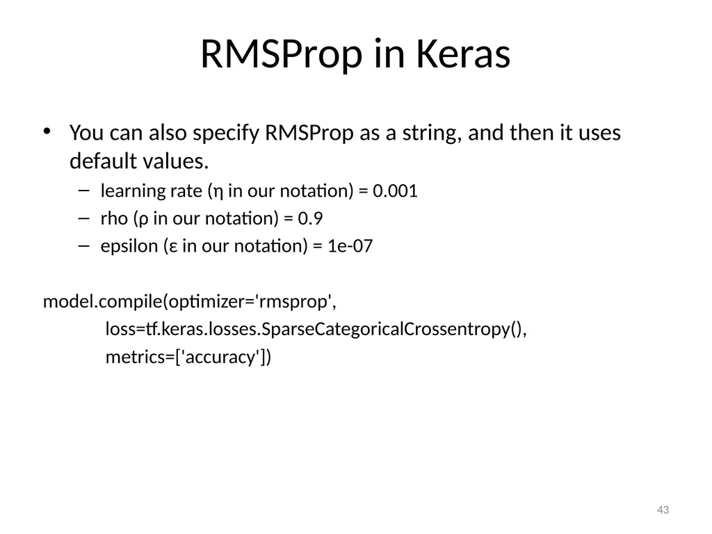
RMSProp in Keras You can also specify RMSProp as a string, and then it uses default values.
learning rate (η in our notation) = 0.001
rho (ρ in our notation) = 0.9
epsilon (ε in our notation) = 1e-07
model.compile(optimizer='rmsprop',
loss=tf.keras.losses.SparseCategoricalCrossentropy(),
metrics=['accuracy']) 43<br>
learning rate (η in our notation) = 0.001
rho (ρ in our notation) = 0.9
epsilon (ε in our notation) = 1e-07
model.compile(optimizer='rmsprop',
loss=tf.keras.losses.SparseCategoricalCrossentropy(),
metrics=['accuracy']) 43<br>
44
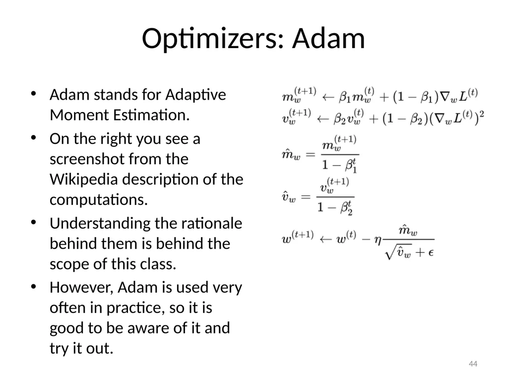
Optimizers: Adam Adam stands for Adaptive Moment Estimation.
On the right you see a screenshot from the Wikipedia description of the computations.
Understanding the rationale behind them is behind the scope of this class.
However, Adam is used very often in practice, so it is good to be aware of it and try it out. 44<br>
On the right you see a screenshot from the Wikipedia description of the computations.
Understanding the rationale behind them is behind the scope of this class.
However, Adam is used very often in practice, so it is good to be aware of it and try it out. 44<br>
45
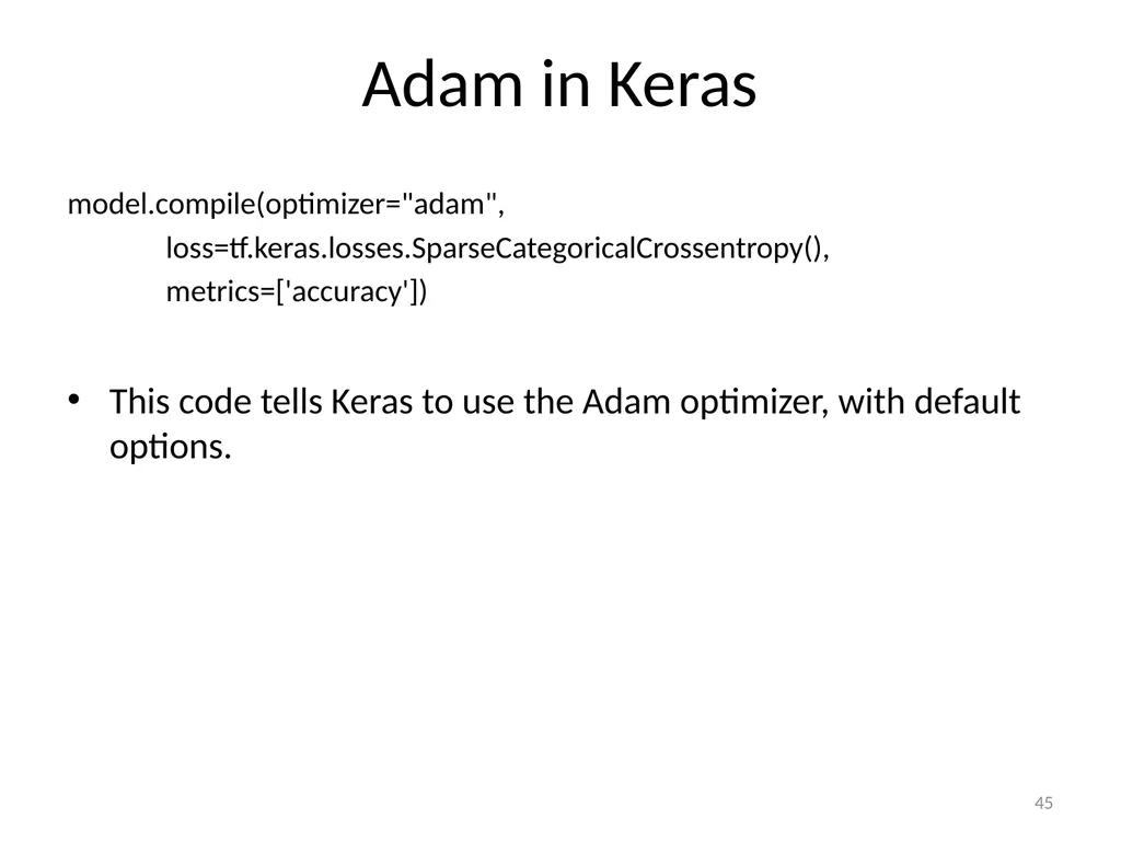
Adam in Keras model.compile(optimizer="adam",
loss=tf.keras.losses.SparseCategoricalCrossentropy(),
metrics=['accuracy'])
This code tells Keras to use the Adam optimizer, with default options. 45<br>
loss=tf.keras.losses.SparseCategoricalCrossentropy(),
metrics=['accuracy'])
This code tells Keras to use the Adam optimizer, with default options. 45<br>
46
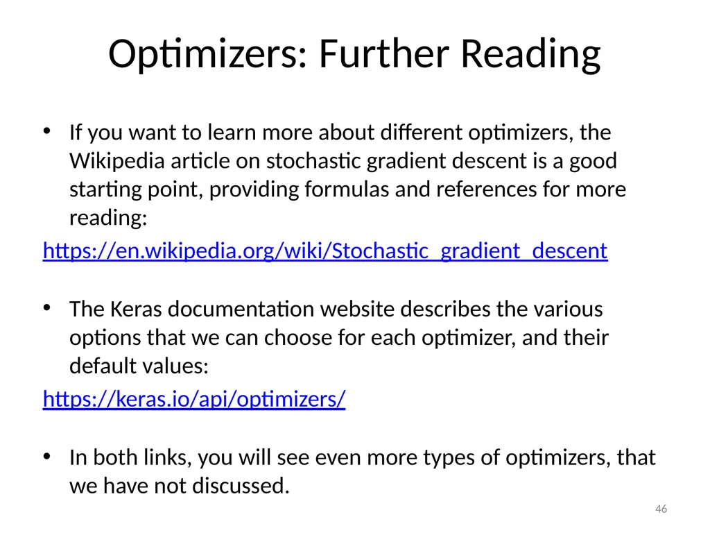
Optimizers: Further Reading If you want to learn more about different optimizers, the Wikipedia article on stochastic gradient descent is a good starting point, providing formulas and references for more reading:
https://en.wikipedia.org/wiki/Stochastic_gradient_descent
The Keras documentation website describes the various options that we can choose for each optimizer, and their default values:
https://keras.io/api/optimizers/
In both links, you will see even more types of optimizers, that we have not discussed. 46<br>
https://en.wikipedia.org/wiki/Stochastic_gradient_descent
The Keras documentation website describes the various options that we can choose for each optimizer, and their default values:
https://keras.io/api/optimizers/
In both links, you will see even more types of optimizers, that we have not discussed. 46<br>
47
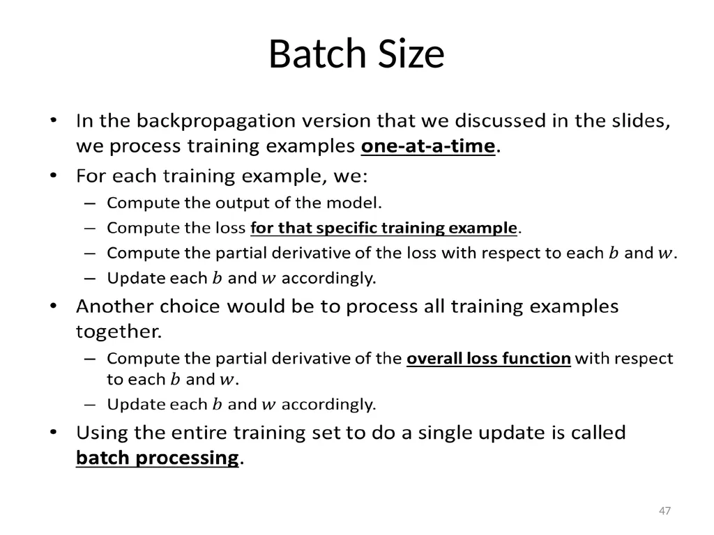
Batch Size 47<br>
48
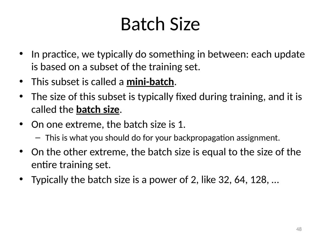
Batch Size In practice, we typically do something in between: each update is based on a subset of the training set.
This subset is called a mini-batch.
The size of this subset is typically fixed during training, and it is called the batch size.
On one extreme, the batch size is 1.
This is what you should do for your backpropagation assignment.
On the other extreme, the batch size is equal to the size of the entire training set.
Typically the batch size is a power of 2, like 32, 64, 128, … 48<br>
This subset is called a mini-batch.
The size of this subset is typically fixed during training, and it is called the batch size.
On one extreme, the batch size is 1.
This is what you should do for your backpropagation assignment.
On the other extreme, the batch size is equal to the size of the entire training set.
Typically the batch size is a power of 2, like 32, 64, 128, … 48<br>
49
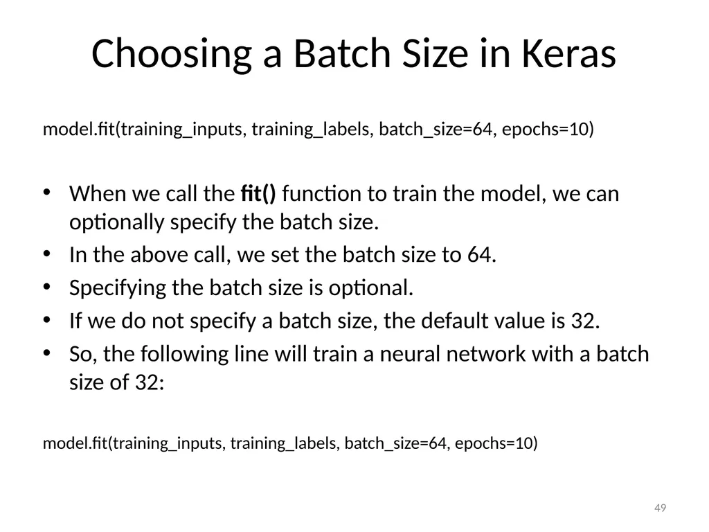
Choosing a Batch Size in Keras model.fit(training_inputs, training_labels, batch_size=64, epochs=10)
When we call the fit() function to train the model, we can optionally specify the batch size.
In the above call, we set the batch size to 64.
Specifying the batch size is optional.
If we do not specify a batch size, the default value is 32.
So, the following line will train a neural network with a batch size of 32:
model.fit(training_inputs, training_labels, batch_size=64, epochs=10) 49<br>
When we call the fit() function to train the model, we can optionally specify the batch size.
In the above call, we set the batch size to 64.
Specifying the batch size is optional.
If we do not specify a batch size, the default value is 32.
So, the following line will train a neural network with a batch size of 32:
model.fit(training_inputs, training_labels, batch_size=64, epochs=10) 49<br>
50
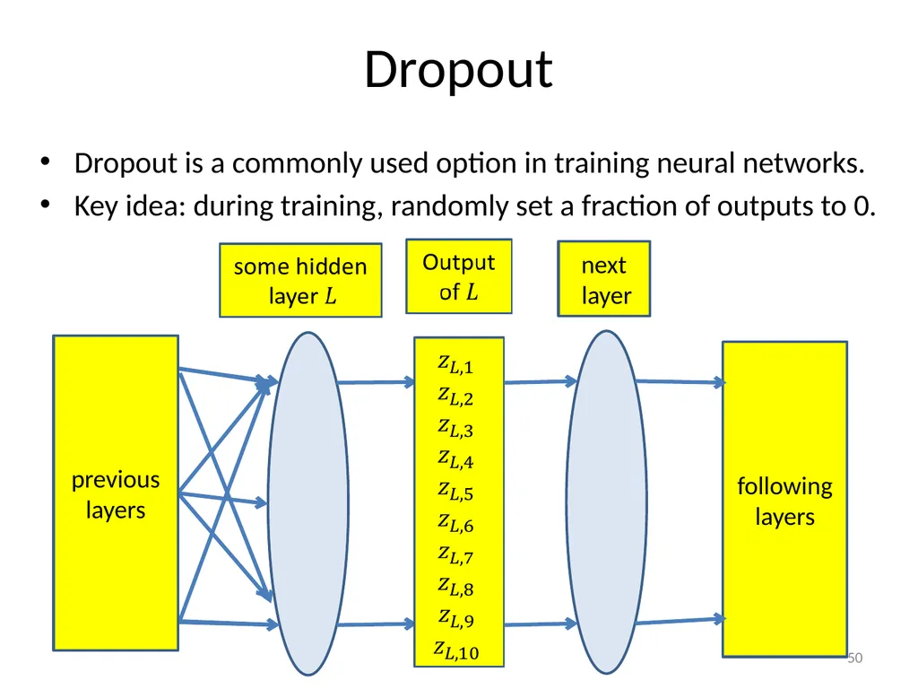
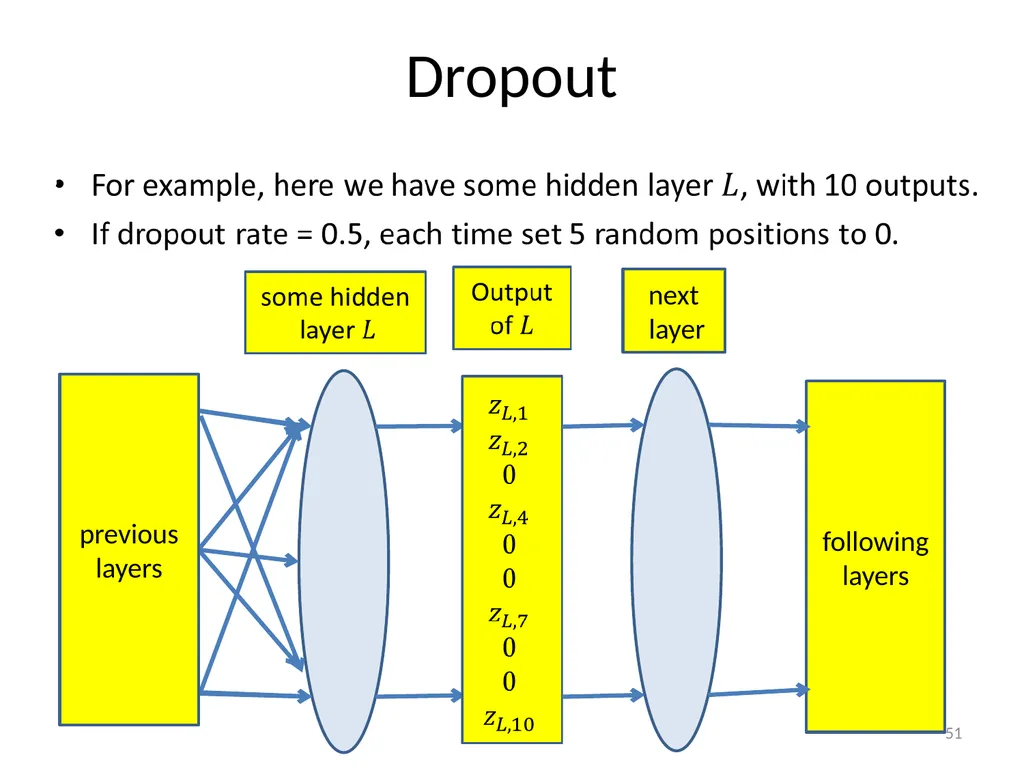
Dropout Dropout is a commonly used option in training neural networks.
Key idea: during training, randomly set a fraction of outputs to 0. 50 previous layers next layer following layers<br>
Key idea: during training, randomly set a fraction of outputs to 0. 50 previous layers next layer following layers<br>
51
Dropout 51 previous layers next
layer following layers<br>
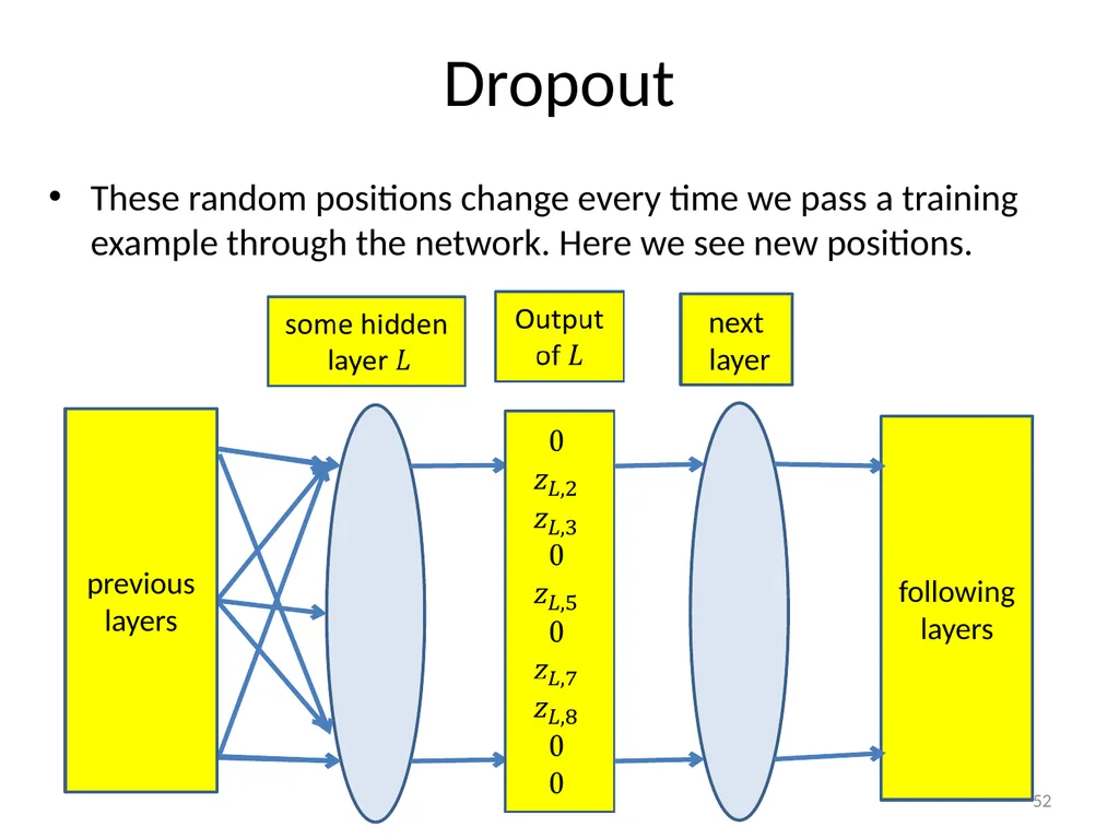
52
Dropout These random positions change every time we pass a training example through the network. Here we see new positions. 52 previous layers next
layer following layers<br>
53
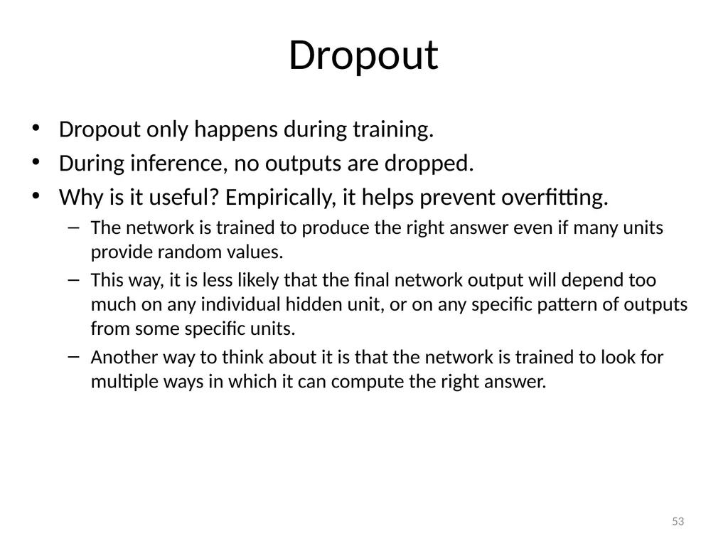
Dropout Dropout only happens during training.
During inference, no outputs are dropped.
Why is it useful? Empirically, it helps prevent overfitting.
The network is trained to produce the right answer even if many units provide random values.
This way, it is less likely that the final network output will depend too much on any individual hidden unit, or on any specific pattern of outputs from some specific units.
Another way to think about it is that the network is trained to look for multiple ways in which it can compute the right answer. 53<br>
During inference, no outputs are dropped.
Why is it useful? Empirically, it helps prevent overfitting.
The network is trained to produce the right answer even if many units provide random values.
This way, it is less likely that the final network output will depend too much on any individual hidden unit, or on any specific pattern of outputs from some specific units.
Another way to think about it is that the network is trained to look for multiple ways in which it can compute the right answer. 53<br>
54
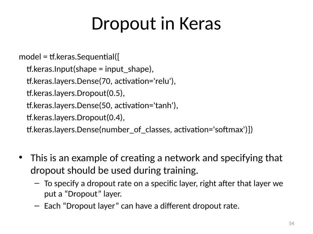
Dropout in Keras model = tf.keras.Sequential([
tf.keras.Input(shape = input_shape),
tf.keras.layers.Dense(70, activation='relu'),
tf.keras.layers.Dropout(0.5),
tf.keras.layers.Dense(50, activation='tanh'),
tf.keras.layers.Dropout(0.4),
tf.keras.layers.Dense(number_of_classes, activation='softmax')])
This is an example of creating a network and specifying that dropout should be used during training.
To specify a dropout rate on a specific layer, right after that layer we put a “Dropout” layer.
Each “Dropout layer” can have a different dropout rate. 54<br>
tf.keras.Input(shape = input_shape),
tf.keras.layers.Dense(70, activation='relu'),
tf.keras.layers.Dropout(0.5),
tf.keras.layers.Dense(50, activation='tanh'),
tf.keras.layers.Dropout(0.4),
tf.keras.layers.Dense(number_of_classes, activation='softmax')])
This is an example of creating a network and specifying that dropout should be used during training.
To specify a dropout rate on a specific layer, right after that layer we put a “Dropout” layer.
Each “Dropout layer” can have a different dropout rate. 54<br>
55
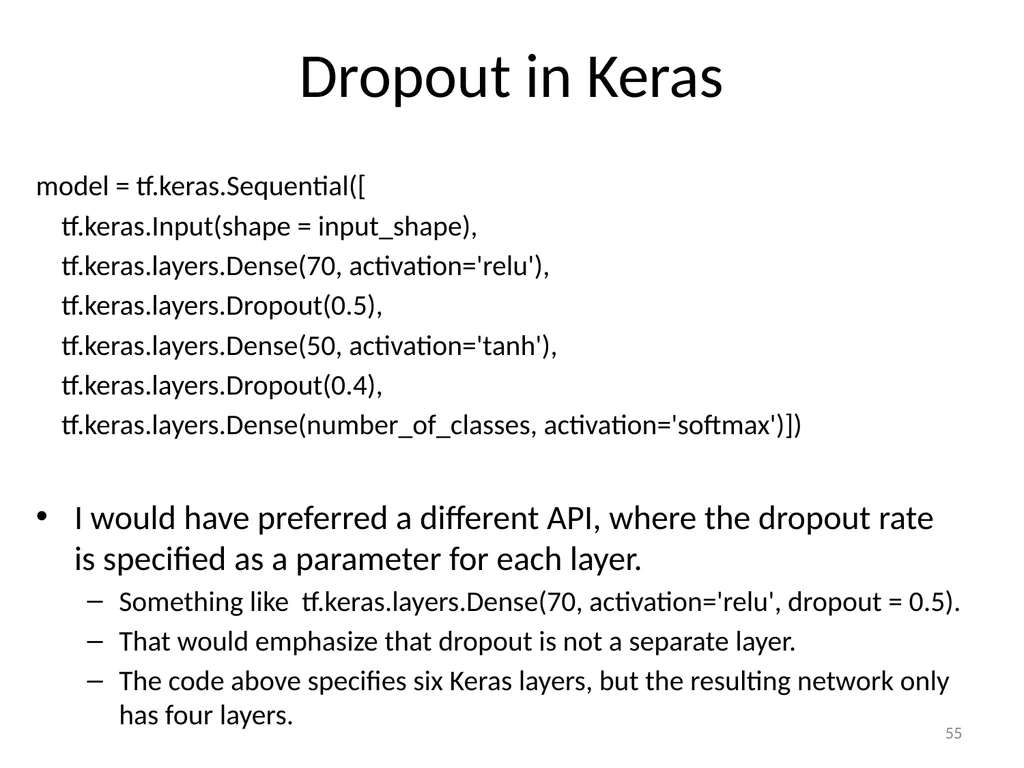
Dropout in Keras model = tf.keras.Sequential([
tf.keras.Input(shape = input_shape),
tf.keras.layers.Dense(70, activation='relu'),
tf.keras.layers.Dropout(0.5),
tf.keras.layers.Dense(50, activation='tanh'),
tf.keras.layers.Dropout(0.4),
tf.keras.layers.Dense(number_of_classes, activation='softmax')])
I would have preferred a different API, where the dropout rate is specified as a parameter for each layer.
Something like tf.keras.layers.Dense(70, activation='relu', dropout = 0.5).
That would emphasize that dropout is not a separate layer.
The code above specifies six Keras layers, but the resulting network only has four layers. 55<br>
tf.keras.Input(shape = input_shape),
tf.keras.layers.Dense(70, activation='relu'),
tf.keras.layers.Dropout(0.5),
tf.keras.layers.Dense(50, activation='tanh'),
tf.keras.layers.Dropout(0.4),
tf.keras.layers.Dense(number_of_classes, activation='softmax')])
I would have preferred a different API, where the dropout rate is specified as a parameter for each layer.
Something like tf.keras.layers.Dense(70, activation='relu', dropout = 0.5).
That would emphasize that dropout is not a separate layer.
The code above specifies six Keras layers, but the resulting network only has four layers. 55<br>
56
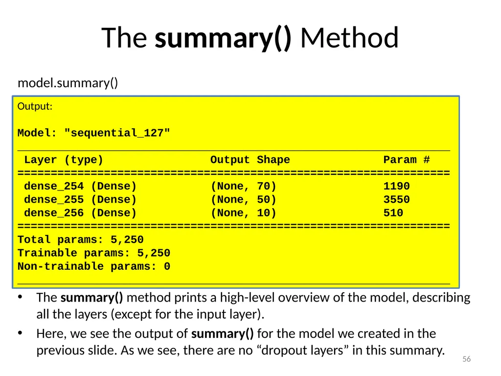
The summary() Method model.summary()
The summary() method prints a high-level overview of the model, describing all the layers (except for the input layer).
Here, we see the output of summary() for the model we created in the previous slide. As we see, there are no “dropout layers” in this summary. 56 Output:
Model: "sequential_127"
_________________________________________________________________
Layer (type) Output Shape Param #
=================================================================
dense_254 (Dense) (None, 70) 1190
dense_255 (Dense) (None, 50) 3550
dense_256 (Dense) (None, 10) 510
=================================================================
Total params: 5,250
Trainable params: 5,250
Non-trainable params: 0
_________________________________________________________________<br>
The summary() method prints a high-level overview of the model, describing all the layers (except for the input layer).
Here, we see the output of summary() for the model we created in the previous slide. As we see, there are no “dropout layers” in this summary. 56 Output:
Model: "sequential_127"
_________________________________________________________________
Layer (type) Output Shape Param #
=================================================================
dense_254 (Dense) (None, 70) 1190
dense_255 (Dense) (None, 50) 3550
dense_256 (Dense) (None, 10) 510
=================================================================
Total params: 5,250
Trainable params: 5,250
Non-trainable params: 0
_________________________________________________________________<br>