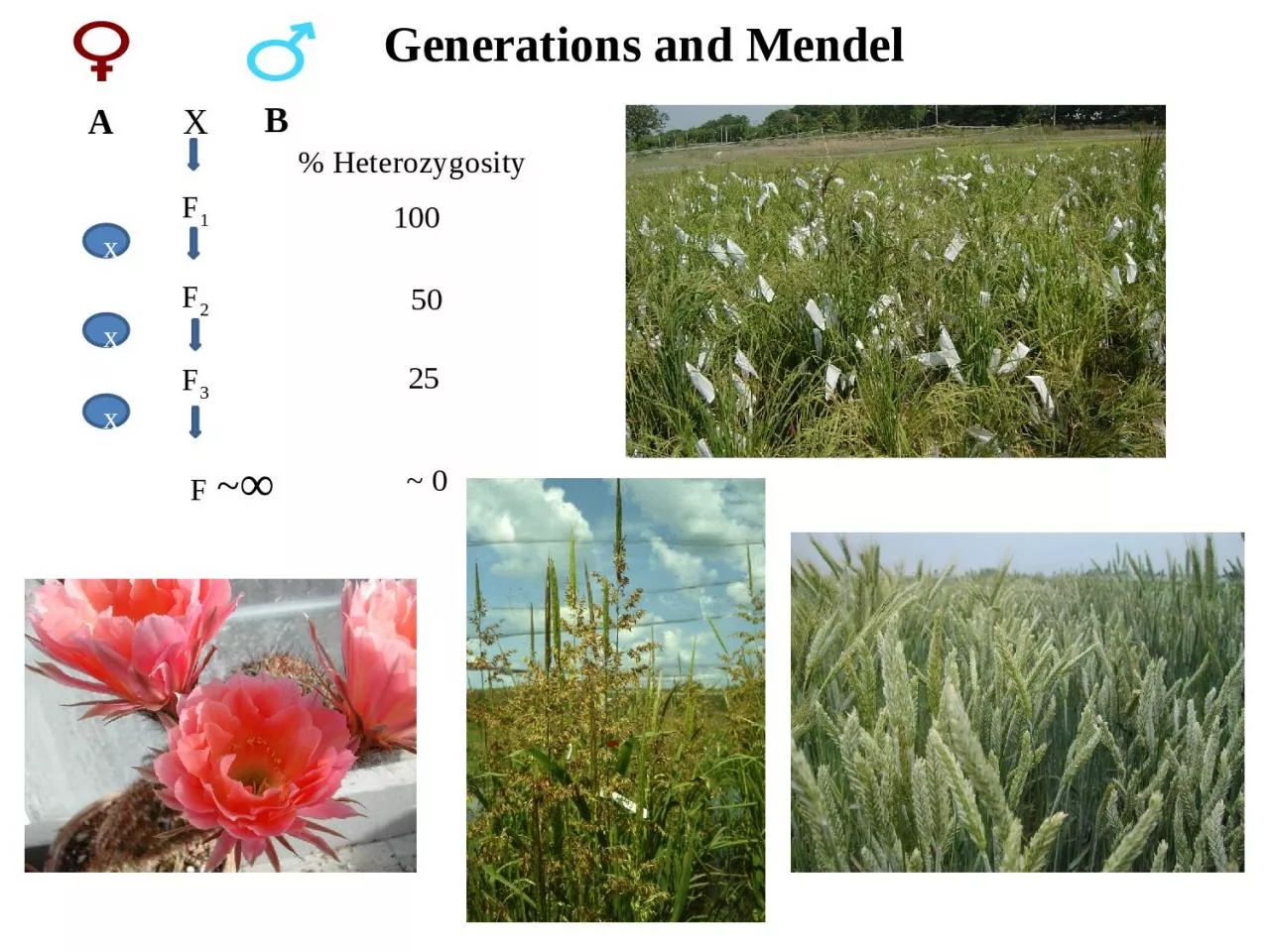
A B F 1 F 2 F 3 F Heterozygosity x x x 100 50 25 0 Generation Advance N n N NN Nn n Nn nn N N N N N N N N N N N N N N N N n n n ID: 934185
Download Presentation The PPT/PDF document "Generations and Mendel X" is the property of its rightful owner. Permission is granted to download and print the materials on this web site for personal, non-commercial use only, and to display it on your personal computer provided you do not modify the materials and that you retain all copyright notices contained in the materials. By downloading content from our website, you accept the terms of this agreement.
Slide1
Generations and Mendel
X
A
B
F
1
F
2
F
3
F
~
∞
% Heterozygosity
x
x
x
100
50
25
~ 0
Slide2Generation
Advance
N
n
N
NN
Nn
n
Nn
nn+
=NN NN N NN NN N NN N NN N
+=nn nN N NN NN N NN N nN n
+=nn nn n nn nn n nn n nn n
+=NN Nn n nn nn n nn n Nn N
Note: At this point in the figure, the antipodals and synergids are deleted and only the fertilized endosperm nuclei (now 3n) and fertilized egg (now 2n) are shown. Only the fertilizedegg is carried to the Punnett square.
Slide3Gregor
Mendel
en.wikipedia.org
https://keen101.wordpress.com/2015/08/19/pea-breeding-resources/
http://www.interactive-biology.com/3813/mendels-pea-plant-experiment-the-root-of-all-in-genetics/
X
A
B
F
1
F
2
F
3
F
~
∞
% Heterozygosity
x
x
x
100
50
25
~ 0
Slide4Crosses between parents generate progeny populations of different types
Filial (F) generations of selfing
Selfing (assuming homozygous parents)
X
A
B
F
1
F
2
F
3
F
~
∞
% Heterozygosity
x
x
x
100
50
25
~ 0
x
Slide5X
A
B
F
1
F
2
F
3
F
~
∞
% Heterozygosity
x
x
x
100
50
25
~ 0
Each plant generation produces seed of the
next generation:
The seed on an F1 plant is F2 seed; the seed
on an F2 plant is F3 seed, etc.
http://www.johnnyseeds.com/flowers/sunflowers/tall-sunflowers/royal-hybrid-1121-sunflower-f1-sunflower-seed-2603.html
Slide6Backcross:
The F1 crossed to either recurrent parent
The number of crosses to the recurrent parent and subsequent cycles of selfing are dictated by experiment/breeding goals
A X B
F
1
X A (or B)
BC1
BC1 X A (B)
BC1
x
x
x
BC2
x
x
BC2 X A (B)
BC3
~ ∞
~ ∞
Slide7Testcross:
A backcross where the recurrent parent is recessive for the target gene(s)
A X B
F
1
X A
BC1
BC1 X A
BC1
x
x
x
BC2
x
x
BC2 X A
BC3
~ ∞
~ ∞
Slide8Recombinant inbred lines:
A cross between two parents, with multiple F2 plants advanced to subsequent generations of selfing to generate
a population of inbred siblings
X
A
B
F
1
F
2
F
3
F
~
∞
x
x
x
….
….
….
….
Slide9Doubled Haploid:
haploid gametes used to generate homozygous 2n plants
A X B
F
1
Gametes
Plants = F ∞
Double chromosome number
….
….
….
….
Slide10Making a cross
Hermaphrodite (barley)
Monoecious (maize)
Dioecious (hops)
Slide11The genetic status (degree of
homozygosity
) of the parents
will determine which generation is appropriate for genetic analysis and the interpretation of the data (e.g. comparison of observed vs. expected phenotypes or genotypes).
Slide12The degree of
homozygosity
of the parents
will likely be a function of their mating biology, e.g. cross vs. self-pollinated.
Slide13Expected and observed ratios in cross progeny will be a function of:
the degree of
homozygosity
of the parents
the generation studied
the degree of dominance
the degree of interaction between genes
the number of genes determining the trait
Slide14Mendelian
analysis
N
n
N
NN
Nn
n
Nnnn
+=NN NN N NN NN N NN N NN N
+=nn nN N NN NN N NN N nN n
+=nn nn n nn nn n nn n nn n
+=NN Nn n nn nn n nn n Nn N
Genetic analysis is straightforward when one or two genes determine the target trait
Slide15Mendelian Inheritance
Mendelian genetic analysis:
The "classical" approach to understanding the
genetic basis of a trait.
Based on analysis of inheritance patterns in the progeny of a cross
R
R
0
R0
R0
0R0R0
R0RRRR00R000
Gregor Mendel
en.wikipedia.orgRR x OO F1 x F2
Slide16R
R
0
R0
R0
0
R0R0
R
0
RRRR00R000
Gregor Mendel
en.wikipedia.orgRoundup Ready (RR) x Organic (OO)F1: RO = Roundup ReadyF2: 1 RR: 2RO: 1OO = 3 Roundup Ready: 1 non-Roundup Ready
Mendelian genetics and transgenic gene flow https://tilth.org/https://www.genuity.com/specialty/Pages/Roundup-Ready-Sugarbeets.aspx
Slide17Mendelian
Qualitative
(discontinuous)
variation
Quantitative
(continuous)
variation
The number of genes determining the trait and/or
The effects of the environment
Parent 1
Parent 2Parent 1Parent 2
Slide18Qualitative Quantitative variation
With just 3 unlinked loci: A B C – start to approach a quantitative distribution
If homozygous for resistance alleles (-) at a locus = 0% contribution to disease severity
Each susceptibility allele (+) at each locus = 10% disease severity
Imagine if there were 10 genes and heterozygotes!
A locus
B locus
C locus Value - -
- -- -
0- - - - + + 20- -+ + - - 20 + +- - - - 20+ + + + - -40+ + - - + + 40- - + + + +40 +++ ++ + 60
Slide19Quantitative Trait Loci
Genetic determinants of quantitative variation
Loci that determine, or are associated with loci that determine,
variation in a phenotype
Slide20Nuclear genome
Autosomal =
Biparental
Sex-linked = XX vs. XY
R
O
R
RRRrORrrrInheritance patterns for polymorphismsXXXXXXXYXY
XYCytoplasmic genomesChloroplasts and mitochondria: ~ uniparental~Maternal in angiosperms~Paternal in gymnosperms Z
ZZ
Slide21Mitochondria
Chloroplast
Cytoplasmic inheritance
Biomedcentral.com
Dombrowski
et al. 1998
Slide22Cytoplasmic inheritance –
origins, function, and important traits
Mitochondria
Once free-living bacteria – now endosymbionts
Respiration
~ 50 genes
Cross talk with nucleus – coevolution and horizontal transfer
Male sterility (cytoplasmic male sterility)Chloroplast Once free-living cyanobacteria– now endosymbionts Photosynthesis Cross talk with nucleus – coevolution and horizontal transfer~ 100 genesVariegation http://www.plantcell.org/content/11/4/571
Slide23Phenotype
2-row
Vrs1
Vrs1
(Or
Vrs1vrs1)
6-row
vrs1vrs1
Mendelian analysis of spike type in barley*
*Autosomal trait
Slide24Genotype
Slide25vrs1
genotypes
Vrs1
phenotypes
Slide26“Six-rowed barley originated from a mutation in a………
homeobox
gene”
Two-rowed
is ancestral (wild type)
Vrs1
Six-rowed
in the mutant
vrs1
Homeobox genes are transcription factorsThe vrs1 (hox1
) model: In a two-row, the product of Vrs1 binds to another (unknown) gene (or genes) that determine the fertility of lateral floretsBy preventing expression of this other gene, lateral florets are sterile and thus the inflorescence has two rows of lateral floretsIn a 6-row (vrs1vrs1) there is a loss of function
Slide27Vrs1
Lat
X
Transcription of
Vrs1
Translation of
Vrs1
Binding of
Vrs1
to
“Lat”*
No expression of
Lat
=2 -row
*
Lat
a hypothetical gene
Slide28vrs1
Lat
X
No transcription of
vrs1
(or)
No translation of
vrs1
No binding of
vrs1
to
“Lat”*
“
Lat
”
expresses and lateral florets are fertile = 6-row
X*Lat a hypothetical gene
Slide29What mutations happened to
Vrs1
to make it
vrs1
(loss of function)?
Complete deletion
of the gene ( - transcription, - translation so no protein)
Deletions of (or insertions into) key regions
of the gene leading to - transcription and/or + transcription but – translation, or incorrect translation
Nucleotide changes leading to + transcription, but incorrect translation leading to non-functional protein
Slide30How many alleles are possible at a locus?
Only two per diploid individual, but many are possible in a population of individuals
New alleles arise through mutation
Some mutations have no discernible effect on phenotype
Different mutations in the same gene may lead to the same or different phenotypes
Slide31OWB-D X OWB-R
F
1
Gametes
Plants = F ∞
Double chromosome number
….
….
….
….
Doubled haploid generation advance
Slide32A quick overview of doubled haploids
F
1
=
Nud
nud
(2n = 2x = 14)
Gametes (male or female)
Nud
nud (n = 7)
Induction/regeneration
Nud
nud
Haploid plantlets (n = 7)
Chromosome doubling (spontaneous/induced)
Mature plants/grain
Nud
Nud
nud
nud
(2n = 2x = 14)
Slide33Anther Culture DH production in barley
Harvest donor spikes
Apply stress conditions
Place anthers on induction medium
Sub-culturing for shoots and roots
Spontaneous doubling
Produce seed Breeding/genetics forever
Slide34OWB dominant x OWB recessive
F1
Doubled haploids
Slide35Hypothesis Testing: Determining the
“
Goodness of Fit
”
Expected and observed ratios in cross progeny will be a function of
the degree of
homozygosity
of the parents
the generation studied the degree of dominance the degree of interaction between genes the number of genes determining the trait
Slide36Hypothesis Testing:
Determining the
“
Goodness of Fit
”
The Chi Square statistic tests "goodness of fit“; that is, how closely observed and predicted results agree
The degrees of freedom that are used for the test are a function of the number of classes
This is a test of a null hypothesis: “the observed ratio and expected ratios are not different
”
Chi square = (O
1
- E
1
)
2
/E1 +........+ (On - E
n)2/E
n
where O1 = number of observed members of the first classE1 = number of expected members of the first class
On = number of observed members of the nth classEn = number of expected members of the nth
class
The Chi square formula
Slide38As deviations from hypothesized ratios get smaller, the chi square value approaches 0; there is a good fit.
As deviations from hypothesized ratios get larger, the chi square value gets larger; there is a poor fit.
What determines good vs. poor?
The probability of observing a deviation as large, or larger, due to chance alone.
p values below 0.05 (i.e. 0.025, 0.01, .005) lie in the area of rejection.
The Chi square concept
Slide39Interpreting the chi square statistic in terms of probability.
Determine degrees of freedom (
df
).
df
= number of classes - 1.
2. Consult chi square table and/or calculator (on web)
Slide40Slide41The data:
Number of kernel rows (
Vrs-1
/
vrs-1
) in barley (
Hordeum vulgare). For simplicity, vrs-1 is abbreviated as "v" in the following table. Hypothesis is 1:1 (expectation for 2 alleles at 1 locus in a doubled haploid population).
Gametes
V
v
DH genotypes VVvv
DH phenotypesTwo-rowSix-row
Number 3547
Chi square computation for a monohybrid ratio
Slide42Phenotype
#Observed
#Expected
O - E
(O - E)
2
/E
VV
35
41
-6
0.89
vv4741
60.89Totals
828201.75 = chi square
Consult table (next slide): p-value (1 df) = 0.18 This chi square is well within the realm of acceptance, so we conclude that there is indeed a 1:1 ratio of two-row: six-row phenotypes in the OWB population.Chi square computation for a monohybrid ratio
Slide43Slide44Chi square computation for dihybrid ratios
Be able to calculate chi-square tests for dihybrid F2, testcross and DH
X
A
B
F
1
F
2
F
3
F
~
∞
% Heterozygosity
x
x
x
100
50
25
~ 0
A X B
F
1
X A
BC1
BC1 X A
BC1
x
x
x
BC2
x
x
BC2 X A
BC3
~ ∞
~ ∞