Linear Filters Monday, Jan 24 - PowerPoint Presentation

348 views
Uploaded On 2020-04-09

Linear Filters Monday, Jan 24 - PPT Presentation

Prof Kristen Grauman UTAustin Announcements Office hours MonThurs 56 pm Mon Yong Jae PAI 533 TuesThurs Shalini PAI 533 Wed Me ACES 3446 cvspring2011csutexasedu for assignment questions outside of office hours ID: 776483

filter source 890 filters filter source 890 filters noise gaussian 910 linear 490 920 image pixel average images filtering

Link:

Copy

Embed:

<iframe width="560" height="315" src="https://www.docslides.com/embed/776483" frameborder="0" allowfullscreen></iframe>

Download Presentation from below link

Download Presentation The PPT/PDF document " Linear Filters Monday, Jan 24" is the property of its rightful owner. Permission is granted to download and print the materials on this web site for personal, non-commercial use only, and to display it on your personal computer provided you do not modify the materials and that you retain all copyright notices contained in the materials. By downloading content from our website, you accept the terms of this agreement.

Presentation Transcript

Slide1

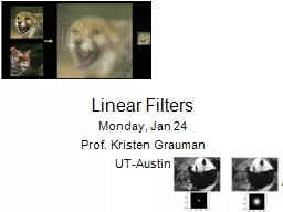
Linear Filters

Monday, Jan 24Prof. Kristen GraumanUT-Austin

…

Slide2

Announcements

Office hours Mon-Thurs 5-6 pmMon: Yong Jae, PAI 5.33Tues/Thurs: Shalini, PAI 5.33Wed: Me, ACES 3.446cv-spring2011@cs.utexas.edu for assignment questions outside of office hoursPset 0 due Friday Jan 28. Drop box in PAI 5.38. Attach cover page with name and CS 376

Slide3

Slide4

Plan for today

Image noise

Linear filters

Examples: smoothing filters

Convolution / correlation

Slide5

Image Formation

Slide credit: Derek Hoiem

Slide6

Digital camera

A digital camera replaces film with a sensor arrayEach cell in the array is light-sensitive diode that converts photons to electronshttp://electronics.howstuffworks.com/digital-camera.htm

Slide by Steve Seitz

Slide7

Slide credit: Derek Hoiem

Digital images

Slide8

Digital images

Sample the 2D space on a regular gridQuantize each sample (round to nearest integer)Image thus represented as a matrix of integer values.

Adapted from S. Seitz

Slide9

Digital color images

Slide10

Color images, RGB color space

Digital color images

Slide11

Images in Matlab

Images represented as a matrixSuppose we have a NxM RGB image called “im”im(1,1,1) = top-left pixel value in R-channelim(y, x, b) = y pixels down, x pixels to right in the bth channelim(N, M, 3) = bottom-right pixel in B-channelimread(filename) returns a uint8 image (values 0 to 255)Convert to double format (values 0 to 1) with im2double

0.920.930.940.970.620.370.850.970.930.920.990.950.890.820.890.560.310.750.920.810.950.910.890.720.510.550.510.420.570.410.490.910.920.960.950.880.940.560.460.910.870.900.970.950.710.810.810.870.570.370.800.880.890.790.850.490.620.600.580.500.600.580.500.610.450.330.860.840.740.580.510.390.730.920.910.490.740.960.670.540.850.480.370.880.900.940.820.930.690.490.560.660.430.420.770.730.710.900.990.790.730.900.670.330.610.690.790.730.930.970.910.940.890.490.410.780.780.770.890.990.93

row

column

Slide credit: Derek Hoiem

Slide12

Image filtering

Compute a function of the local neighborhood at each pixel in the imageFunction specified by a “filter” or mask saying how to combine values from neighbors.Uses of filtering:Enhance an image (denoise, resize, etc)Extract information (texture, edges, etc)Detect patterns (template matching)

Adapted from Derek Hoiem

Slide13

Motivation: noise reduction

Even multiple images of the

same static scene

will not be identical.

Slide14

Common types of noise

Salt and pepper noise: random occurrences of black and white pixelsImpulse noise: random occurrences of white pixelsGaussian noise: variations in intensity drawn from a Gaussian normal distribution

Source: S. Seitz

Slide15

Gaussian noise

Fig: M. Hebert

>> noise = randn(size(im)).*sigma;

>> output = im + noise;

What is impact of the sigma?

Slide16

Motivation: noise reduction

Even multiple images of the same static scene will not be identical.

How could we reduce the noise, i.e., give an estimate of the true intensities?

What if there’s only one image?

Slide17

First attempt at a solution

Let’s replace each pixel with an average of all the values in its neighborhood

Assumptions:

Expect pixels to be like their neighbors

Expect noise processes to be independent from pixel to pixel

Slide18

First attempt at a solution

Let’s replace each pixel with an average of all the values in its neighborhoodMoving average in 1D:

Source: S. Marschner

Slide19

Weighted Moving Average

Can add weights to our moving averageWeights [1, 1, 1, 1, 1] / 5

Source: S. Marschner

Slide20

Weighted Moving Average

Non-uniform weights [1, 4, 6, 4, 1] / 16

Source: S. Marschner

Slide21

Moving Average In 2D

00000000000000000000000909090909000000909090909000000909090909000000900909090000009090909090000000000000009000000000000000000

00000000000000000000909090909000000909090909000000909090909000000900909090000009090909090000000000000009000000000000000000

Source: S. Seitz

Slide22

Moving Average In 2D

00000000000000000000000909090909000000909090909000000909090909000000900909090000009090909090000000000000009000000000000000000

000000000000000000000909090909000000909090909000000909090909000000900909090000009090909090000000000000009000000000000000000

Source: S. Seitz

Slide23

Moving Average In 2D

00000000000000000000000909090909000000909090909000000909090909000000900909090000009090909090000000000000009000000000000000000

1020

000000000000000000000909090909000000909090909000000909090909000000900909090000009090909090000000000000009000000000000000000

Source: S. Seitz

Slide24

Moving Average In 2D

00000000000000000000000909090909000000909090909000000909090909000000900909090000009090909090000000000000009000000000000000000

102030

000000000000000000000909090909000000909090909000000909090909000000900909090000009090909090000000000000009000000000000000000

Source: S. Seitz

Slide25

Moving Average In 2D

010203030

000000000000000000000909090909000000909090909000000909090909000000900909090000009090909090000000000000009000000000000000000

Source: S. Seitz

Slide26

Moving Average In 2D

00000000000000000000000909090909000000909090909000000909090909000000900909090000009090909090000000000000009000000000000000000

203030302010020406060604020030609090906030030508080906030030508080906030020305050604020102030303030201010101000000

Source: S. Seitz

Slide27

Correlation filtering

Say the averaging window size is 2k+1 x 2k+1:

Loop over all pixels in neighborhood around image pixel F[i,j]

Attribute uniform weight to each pixel

Now generalize to allow

different weights

depending on neighboring pixel’s relative position:

Non-uniform weights

Slide28

Correlation filtering

Filtering an image: replace each pixel with a linear combination of its neighbors.

The filter “kernel” or “mask” H[u,v] is the prescription for the weights in the linear combination.

This is called

cross-correlation

, denoted

Slide29

Averaging filter

What values belong in the kernel H for the moving average example?

010203030

000000000000000000000909090909000000909090909000000909090909000000900909090000009090909090000000000000009000000000000000000

“box filter”

Slide30

Smoothing by averaging

depicts box filter:

white = high value, black = low value

original

filtered

What if the filter size was 5 x 5 instead of 3 x 3?

Slide31

Boundary issues

What is the size of the output?

MATLAB: output size / “shape” optionsshape = ‘full’: output size is sum of sizes of f and gshape = ‘same’: output size is same as fshape = ‘valid’: output size is difference of sizes of f and g

full

same

valid

Source: S. Lazebnik

Slide32

Boundary issues

What about near the edge?the filter window falls off the edge of the imageneed to extrapolatemethods:clip filter (black)wrap aroundcopy edgereflect across edge

Source: S. Marschner

Slide33

Boundary issues

What about near the edge?the filter window falls off the edge of the imageneed to extrapolatemethods (MATLAB):clip filter (black): imfilter(f, g, 0)wrap around: imfilter(f, g, ‘circular’)copy edge: imfilter(f, g, ‘replicate’)reflect across edge: imfilter(f, g, ‘symmetric’)

Source: S. Marschner

Slide34

Gaussian filter

0000000000000000000000909090909000000909090909000000909090909000000900909090000009090909090000000000000009000000000000000000

121242121

What if we want nearest neighboring pixels to have the most influence on the output?

Removes high-frequency components from the image (“low-pass filter”).

This kernel is an approximation of a 2d Gaussian function:

Source: S. Seitz

Slide35

Smoothing with a Gaussian

Slide36

Gaussian filters

What parameters matter here?Size of kernel or maskNote, Gaussian function has infinite support, but discrete filters use finite kernels

= 5 with 10 x 10 kernel

= 5 with 30 x 30 kernel

Slide37

Gaussian filters

What parameters matter here?

Variance of Gaussian: determines extent of smoothing

= 2 with 30 x 30 kernel

= 5 with 30 x 30 kernel

Slide38

Matlab

>> hsize = 10;>> sigma = 5;>> h = fspecial(‘gaussian’ hsize, sigma);>> mesh(h);>> imagesc(h);>> outim = imfilter(im, h); % correlation >> imshow(outim);

outim

Slide39

Smoothing with a Gaussian

for sigma=1:3:10

h = fspecial('gaussian‘, fsize, sigma);

out = imfilter(im, h); imshow(out); pause; end

…

Parameter

is the “scale” / “width” / “spread” of the Gaussian kernel, and controls the amount of smoothing.

Slide40

Properties of smoothing filters

Smoothing

Values positive

Sum to 1



constant regions same as input

Amount of smoothing proportional to mask size

Remove “high-frequency” components; “low-pass” filter

Slide41

Filtering an impulse signal

0000000000000000000000001000000000000000000000000

abcdefghi

What is the result of filtering the impulse signal (image)

with the arbitrary kernel

Slide42

Convolution

Convolution: Flip the filter in both dimensions (bottom to top, right to left)Then apply cross-correlation

Notation for convolution operator

Slide43

Convolution vs. correlation

Convolution

Cross-correlation

For a Gaussian or box filter, how will the outputs differ?

If the input is an impulse signal, how will the outputs differ?

Slide44

Predict the outputs using correlation filtering

= ?

Slide45

Practice with linear filters

Original

Source: D. Lowe

Slide46

Practice with linear filters

Original

Filtered

(no change)

Source: D. Lowe

Slide47

Practice with linear filters

Original

Source: D. Lowe

Slide48

Practice with linear filters

Original

Shifted left

by 1 pixel with correlation

Source: D. Lowe

Slide49

Practice with linear filters

Original

Source: D. Lowe

Slide50

Practice with linear filters

Original

Blur (with a

box filter)

Source: D. Lowe

Slide51

Practice with linear filters

Original

Source: D. Lowe

Slide52

Practice with linear filters

Original

Sharpening filter:

accentuates differences with local average

Source: D. Lowe

Slide53

Filtering examples: sharpening

Slide54

Properties of convolution

Shift invariant:

Operator behaves the same everywhere, i.e. the value of the output depends on the pattern in the image neighborhood, not the position of the neighborhood.

Superposition:

h * (f1 + f2) = (h * f1) + (h * f2)

Slide55

Properties of convolution

Commutative:

f * g = g * f

Associative

(f * g) * h = f * (g * h)

Distributes over addition

f * (g + h) = (f * g) + (f * h)

Scalars factor out

kf * g = f * kg = k(f * g)

Identity:

unit impulse e = […, 0, 0, 1, 0, 0, …]. f * e = f

Slide56

Separability

In some cases, filter is separable, and we can factor into two steps:

Convolve all rows

Convolve all columns

Slide57

Separability

In some cases, filter is separable, and we can factor into two steps: e.g.,

What is the computational complexity advantage for a separable filter of size k x k, in terms of number of operations per output pixel?

f * (g * h) = (f * g) * h

Slide58

Effect of smoothing filters

Additive Gaussian noise

Salt and pepper noise

Slide59

Median filter

No new pixel values introduced

Removes spikes: good for impulse, salt & pepper noise

Non-linear filter

Slide60

Median filter

Salt and pepper noise

Median filtered

Source: M. Hebert

Plots of a row of the image

Matlab: output im = medfilt2(im, [h w]);

Slide61

Median filter

Median filter is edge preserving

Slide62

Aude Oliva & Antonio Torralba & Philippe G Schyns, SIGGRAPH 2006

Filtering application: Hybrid Images

Slide63

Application: Hybrid Images

Gaussian Filter

Laplacian Filter

A. Oliva, A. Torralba, P.G. Schyns,

“Hybrid Images,”

SIGGRAPH 2006

Gaussian

unit impulse

Laplacian of Gaussian

Slide64

Aude Oliva & Antonio Torralba & Philippe G Schyns, SIGGRAPH 2006

Slide65

Aude Oliva & Antonio Torralba & Philippe G Schyns, SIGGRAPH 2006

Slide66

Summary

Image “noise”

Linear filters and convolution useful for

Enhancing images (smoothing, removing noise)

Box filter

Gaussian filter

Impact of scale / width of smoothing filter

Detecting features (next time)

Separable filters more efficient

Median filter: a non-linear filter, edge-preserving

Slide67

Coming up

Wednesday:

Filtering part 2: filtering for features

Friday:

Pset 0 is due via turnin, 11:59 PM

Linear Filters Monday, Jan 24 - PowerPoint Presentation

Linear Filters Monday, Jan 24 - PPT Presentation

Share:

Link:

Embed:

Related Contents