/
Mantle Mantle

Mantle - PowerPoint Presentation

cheryl-pisano
cheryl-pisano . @cheryl-pisano
Follow
416 views
Uploaded On 2015-10-26

Mantle - PPT Presentation

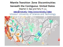
Transition Zone Discontinuities beneath the Contiguous United States Stephen S Gao and Kelly H Liu sgaomstedu httpwwwmstedusgao Missouri University of Science and Technology ID: 172920

mtz 660 mantle velocity 660 mtz velocity mantle 410 depths zone beneath model areas hot gao upper discontinuities transition

Share:

Link:

Embed:

Download Presentation from below link

Download Presentation The PPT/PDF document "Mantle" is the property of its rightful owner. Permission is granted to download and print the materials on this web site for personal, non-commercial use only, and to display it on your personal computer provided you do not modify the materials and that you retain all copyright notices contained in the materials. By downloading content from our website, you accept the terms of this agreement.


Presentation Transcript

Slide1

Mantle

Transition Zone Discontinuities beneath the Contiguous United StatesStephen S. Gao and Kelly H. Liusgao@mst.edu; http://www.mst.edu/~sgao Missouri University of Science and Technology

1Slide2

The mantle transition zone (MTZ) is the region between the 410 and 660 km discontinuities.Variations of the depths are indicators of temperature and water content in the vicinity of the discontinuities.The cartoon was modified from

Foulger and Julian, 2004 (http://www.mantleplumes.org) and Deuss, 2007.2

o

r hydration

(c) Very hot regimes

660

660Slide3

Total number of RFs used in the study: about

310,000 recorded over 25 years till late 2013Small black triangles: 2848 broadband seismic stations used in the studyColor of image: number of P-to-S receiver functions in radius=1o circles L

arge

red

triangles: Previously proposed

hot spots (YS: Yellowstone, RT: Raton, and BMD:

Bermuda)

T

hick black lines

outline major tectonic provinces

(After Gao and Liu, 2014a, JGR)

3Slide4

Spatial

distribution of earthquake source areas. Total number of events used in the study: 6315Each dot represents a radius = 1 degree circular area. The distance between neighboring circular areas is 1 degree. The color of the dot represents the number of used receiver functions originated from earthquakes in the circle. Note the nonlinear nature of the scale bar.

4Slide5

Receiver function stacking procedure (following the approach of Gao and Liu, 2014b, EPSL)Before the computation of the receiver functions, we reduce the degenerating effects of the strong PP arrivals by applying the following exponential function:

5Slide6

Receiver function stacking under the non-plane wave assumption For each candidate depth (from 0 to 800 km),

moveout correct and stack the RFs under the non-plane wave assumption (in which the ray-parameters of the direct P and the P-to-S converted phases are different):6Slide7

Example depth

series along four E-W profiles. Each trace is the result of stacking of RFs with piercing points (at 535 km depth) in radius=1 degree circles.Marked features are as follows: I: Juan de Fuca slab;II: Yellowstone; III: proposed lithospheric drip beneath the northern Basin and Range Province [West et al., 2009]; IV

:

d410 uplift

beneath the southern Colorado Plateau.

7Slide8

Results

of RF stacking based on the 1-D IASP91 Earth model: (a) Apparent 410 depths;(b) Apparent 660 depths;(c) Apparent MTZ thickness.Note that in (c), the colored areas have a MTZ thickness that differs from the IASP91 value of 250 km by 5 km or greater.

8Slide9

The apparent depths of the 410 are highly correlated with those of the 660, indicating that the bulk of the variations is velocity perturbations in the upper mantle.

9Slide10

Unless we accept the unlikely assumption that most of the study area has a very hot MTZ, the true depths of the 410 and 660 should be negatively correlated and not positively correlated.

10660660

o

r hydration

(c) Very hot regimes

660

660Slide11

We next try to construct an S-wave model using MIT13p (Burdick et al., 2014) for depth correction.

For each candidate gamma value which is dln(Vs)∕dln(Vp)we take the MIT13p model and derive an Vs model, and make velocity corrections to the depths. The figure shows cross-correlation coefficients between corrected 410 and 660 depths plotted against the candidate gamma values.

The optimal

gamma

value corresponding to

the minimum XCC is 2.15 for the WUS and 1.70 for the CEUS.

11Slide12

Corrected 410

depths versus corrected 660 depths, using the optimal gamma values.Note the significant reductions of the absolute value of the XCC relative to the uncorrected situation.12Slide13

Corrected 410

and 660 depths using MITP13 and the optimal gamma values. The triangles represent proposed hot spots, and the ellipse outlines the portion of the Juan de Fuca slab in the MTZ. NMSZ: New Madrid Seismic Zone.13Slide14

Main observationsStatistically, both the WUS and CEUS have a MTZ thickness that is within a few km from the global mean of 250 km: Meaning that most tectonic differences between the 2 areas are limited in the upper mantleThe MTZ adjacent to the Pacific plate is hotter than normal, due to 410 depression

The Juan de Fuca slab interacts with the MTZ beneath the Rocky Mountain FrontCold Farallon slabs may exist in the MTZ beneath central US, consistent with previous results (e.g., Porritt et al., 2014; Sigloch, 2011; Pavlis et al., 2012)14Slide15

Main observations The Yellowstone and Raton areas have normal MTZ thickness: Perhaps they are upper mantle features? The Bermuda has a depressed 410 but normal 660. Results of limited data, or a hot feature that extends to the upper MTZ?

15Slide16

The key to resolve the plume-or-not issue using MTZ measurements:Accurate seismic velocity models for both P- and S-wavesHow to create a “perfect” mantle plume?

The true situation: Perfectly normal depths and velocities16Mohamed et al., 2014 GJISlide17

If a low velocity zone is artificially introduced in the MTZ, the 660 would uplift after velocity corrections using the wrong velocity model.

17Slide18

If a high velocity zone is artificially introduced in the upper mantle, both the 410 and 660 would depress after velocity corrections using the wrong velocity model.

18Slide19

If a high velocity zone is artificially introduced in the upper mantle, AND a LVZ is artificially introduced in the MTZ, the 410 would depress and the 660 would uplift after velocity corrections using the wrong velocity model.

19Slide20

Given the limited vertical resolution of (mostly body-wave) tomography techniques, AND the need to balance the total travel-times, the above artificial velocity anomalies are quite possible …, resulting in a thinned MTZ with low velocities – A “perfect” but fake plume coming from the lower mantle!!

20Slide21

For more infoGao, S. S., and K.H. Liu (2014a), Mantle transition zone discontinuities beneath the contiguous United States,

Journal of Geophysical Research Gao, S.S., and K.H. Liu (2014b), Imaging mantle transition zone discontinuities using multiply reflected P-to-S conversions, Earth & Planetary Science LettersMohamed, A.A., S.S. Gao, A.A. Elsheikh, K.H. Liu, Y. Yu, and R.E. Fat-Helbary (2014), Seismic imaging of mantle transition zone discontinuities beneath the northern Red Sea and adjacent areas, Geophysical Journal International 21