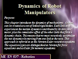
Purpose This chapter introduces the dynamics of mechanisms A robot can be treated as a set of linked rigid bodies Each link body experiences the motion dynamics contributed by its own joint motor plus the cumulative effect of the other links that form a dynamic chain This means that we must ID: 337679
Download Presentation The PPT/PDF document "Dynamics of Robot Manipulators" is the property of its rightful owner. Permission is granted to download and print the materials on this web site for personal, non-commercial use only, and to display it on your personal computer provided you do not modify the materials and that you retain all copyright notices contained in the materials. By downloading content from our website, you accept the terms of this agreement.
Slide1
Dynamics of Robot Manipulators
Purpose:
This chapter introduces the dynamics of mechanisms. A robot can be treated as a set of linked rigid bodies. Each link body experiences the motion dynamics contributed by its own joint motor plus the cumulative effect of the other links that form a dynamic chain. This means that we must recursively accumulate the net dynamics by moving from one link to the next. This approach is referred to as the Newton-Euler recursive equations. The equation types are distinguished as Newton for force equations and as Euler for moment equations. Slide2
In particular, you will
Review the fundamental force and moment equations for rigid bodies.
Determine that the moment of forces applied to a rigid body is the rate of change of angular momentum if taken about the body’s center of mass or about an inertial point.
Apply Newton-Euler recursive equations for the connected rigid links of a mechanism.
Understand that forward recursion is used to propagate motion through the links, while backward recursion is used to propagate forces and torques through the links.Slide3
Review of fundamental equations
Given a system of particles
translating through space,
each particle i being acted
upon by external force F
i
, and
each particle located relative to an inertial reference frame, the governing equations are Fc = m ac (6.10) M = (6.11) Mc = c (6.12)
What is an inertial frame?Slide4
Review of fundamental equations
where
m = total mass (sum over all mass particles)
a
c
= acceleration of center of mass (cm) of all mass particles
F
c = sum of external forces applied to system of particles as if applied at cm Hi = ri x mivi = angular momentum of particle i (also called moment of momentum) H, Hc = angular momentum summed over all particles, measured about inertial point, cm point, respectively M, Mc = moment of all external forces applied to system of particles, measured about inertial point, cm point, respectivelySlide5
Rigid bodies in general motion
(translating and rotating)
Z
X
Y
x
y
z
a
w
The time rate of change of any vector V capable of being viewed
in either XYZ or xyz is
[ ]
XYZ
=
[ ]
xyz
+
w
x
V
where
w
is the angular velocity of a secondary translating, rotating reference frame (xyz).Slide6
Rigid bodies in general motion
(translating and rotating)
Z
X
Y
x
y
z
a
w
Another common form of the
equation is:
=
r
+
w
x
V (6.13)
and when applied to rate of change
of angular momentum becomes
M
= =
r
+
w
x
H (6.16)
which is referred to as Euler’s equation.
Slide7
Rotating rigid body
By integrating the motion over the rigid body, we can express the
angular momentum relative
to the xyz axes as
H = H
x
i + H
y j + Hz k = (Jxx wx + Jxy wy + Jxz
wz
) i + (Jyx wx
+ Jyy w
y + Jyz wz
) j
+ (J
zx
w
x
+ J
zy
w
y
+ J
zz
w
z
) k
(6.20)
or in matrix form
H
=
J
wwhere J = inertia matrixmomentsproductsSlide8
Rotating rigid body
Taking the derivative of (6.20) and substituting into (6.16), also assuming the body axes to be aligned with the
principal axes
, we get Euler’s moment equations:
M
x
= J
xx
x + (Jzz - Jyy) wy wz (6.29a) My
= Jyy y
+ (Jxx - Jzz) w
x w
z (6.29b) Mz = Jzz
z
+ (J
yy
- J
xx
)
w
x
w
y
(6.29c)
What are principal axes?Slide9
Acceleration relative to a non-inertial reference frame
y
x
z
X
Y
Z
w
a
P
r
R
rSlide10
Acceleration relative to a non-inertial reference frame
By taking two derivatives and applying (6.13) appropriately, the absolute acceleration of point P can be shown to be
a
=
+
a
x r + w x (w x r) + + 2 w x (6.31) where = acceleration of xyz origin a
x r = tangential acceleration
w x (w x r
) = centripetal acceleration = acceleration of P relative to xyz 2
w x = Coriolis acceleration Slide11
Acceleration relative to a non-inertial reference frame
For the special case of xyz fixed to rigid body and P a point in the body, and (6.31) reduces to
a = +
a
x
r
+ w x (w x r) (6.32) If P at cm, then ac = +
a x rc
+ w x (w
x rc
) (6.33)Slide12
Recursive Newton-Euler Equations
(forward recursion for motion)
Use Craig/Red D-H formSlide13
Recursive Newton-Euler Equations
If v
i
=
i
and
w
i
is defined to be the angular velocity of the ith joint frame xi yi zi with respect to base coordinates, then where describes the velocity of xi+1, yi+1, zi+1 relative to an observer in frame xi, yi, zi. Slide14
Recursive Newton-Euler Equations
Likewise, the acceleration becomes
Defining
w
i+1
to be the absolute angular velocity of the i+1
frame and
to be the angular velocity of the i+1 frame relative to the ith frame: Slide15
Recursive Newton-Euler Equations
Taking one more derivative for angular acceleration:Slide16
Recursive Newton-Euler Equations
Now applying the DH coordinate representation for manipulators: Slide17
Recursive Newton-Euler Equations
Using the previous equations, we can generate the angular motion recursive equations:Slide18
Recursive Newton-Euler Equations
The linear velocity and acceleration equations use the D-H forms:
where
i+1
is the translational velocity of x
i+1
, y
i+1
, zi+1 relative to xi , yi , zi Slide19
Recursive Newton-Euler Equations
Substituting (6.59) – (6.62), we get the velocity and acceleration recursion equations:
Note that
w
i+1
=
w
i
for translational link i+1.Slide20
Recursive Newton-Euler Equations
(backward recursion for forces and torques)
X
o
Y
o
Z
o
Joint i+1
Link i
N
i
p
i
F
i
r
i
,
w
i
*
z
w
i
z
i+1
i
w
i
.
c
iSlide21
Recursive Newton-Euler Equations
(backward recursion for forces and torques)
Link i
n
i
f
i
f
i+1
n
i+1
Joint Forces/TorquesSlide22
Recursive Newton-Euler Equations
Define the terms:
m
i
= mass of link i
r
i
= position of link i cm with respect to base coordinates
Fi = total force exerted on link i Ni = total moment " " " " * Ji = inertia matrix of link i about its cm determined in the Xo Yo Zo axes
fi = force exerted on link i by link i-1
ni = moment " " " “Slide23
Recursive Newton-Euler Equations
For each link we must apply the N-E equations:
The gravitational acceleration and damping torques will be added to the equations of motion later. Slide24
Recursive Newton-Euler Equations
Now
i
is easily calculated by knowing the acceleration of the origin of the i
th
frame attached to link i at joint i. We locate link i cm with respect to x
i
y
i zi by ci such that ri = ci + pi. The velocity of the cm of link i is obviously Slide25
Recursive Newton-Euler Equations
To determine F
i
and N
i
define
f
i = force exerted on link i by link i-1 ni = moment " " " “Then Fi = fi – fi+1 (6.71)and Ni = ni
– ni+1 + (pi
- ri ) x fi - (pi+1 - r
i ) x fi+1
(6.72) = ni – ni+1 - c
i
x F
i
– s
i+1
x f
i+1
Slide26
Recursive Newton-Euler Equations
The previous equations can be placed in the backwards recursion form to work from the forces/moments exerted on the hand backwards to the joint torques necessary to react to these hand interactions and move the manipulator:
f
i
= f
i+1
+ F
i (6.74) ni = ni+1 + ci x Fi + si+1 x fi+1 + Ni
(6.75) Slide27
Recursive Newton-Euler Equations
The motor torque
t
i
required at joint i is the sum of the joint torque n
i
resolved along the revolute axis plus the damping torque,
ti = ni ˙ zi + bi i (revolute) (6.76a) where bi is the damping coefficient.
For a translational joint
ti = li fi
˙zi
+ bi i (translational) (6.77a)
where
l
i
is the torque arm for motor i. Slide28
And what about gravity?
The effect of gravity on each link is accounted for by applying a base acceleration equal to gravity to the base frame of the robot:
o
= g z
o
with z
o
vertical.
o is applied to the base link in equations (6.65) and (6.66) for i = 0 and this serves to transmit the acceleration of gravity to each link by recursion. Slide29
There are two basic problems with the derivation so far. What are they?
Problem 1
- J
i
in (6.68) when resolved into base coordinates is a function of manipulator configuration. To avoid this unnecessary complexity, we apply the equations at the cm of each link where J
i
is constant.
Problem 2
– The recursive relations have not resolved the various vectors from one joint frame to the next. We must adjust the equations accordingly. Slide30
Do we use the full homogeneous transformation in the recursive equations?
We resolve the free vectors by applying the rotational sub-matrix of the D-H transformations for each joint frame to the recursive vectors, using the Craig/Red D-H representation. Let us also use Tsai’s notation.
joint frame i+1 relative to joint frame i:
joint frame i relative to joint frame i+1:Slide31
Revised angular motion equations
Do you notice anything about the form of the D-H rotational sub-matrix?Slide32
Revised linear motion equationsSlide33
Revised force and torque equationsSlide34
Dynamics summary
The N-E equations are applied recursively to generate the forces and torques at each joint motor. We first apply forward recursion to get the motion state for each link. We then use this motion state to propagate the forces and torques in backward recursion to each joint. The rotational sub-matrix of the D-H transformations must be applied to resolve the vectors correctly into each link’s joint frame
.