/
Short-range forecast Short-range forecast

Short-range forecast - PowerPoint Presentation

karlyn-bohler
karlyn-bohler . @karlyn-bohler
Follow
348 views
Uploaded On 2020-01-18

Short-range forecast - PPT Presentation

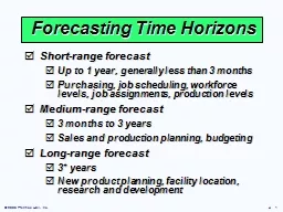
Shortrange forecast Up to 1 year generally less than 3 months Purchasing job scheduling workforce levels job assignments production levels Mediumrange forecast 3 months to 3 years Sales and production planning budgeting ID: 773142

sales deviation forecast demand deviation sales demand forecast error actual signal 100 correlation variable payroll tracking 110 140 squares

Share:

Link:

Embed:

Download Presentation from below link

Download Presentation The PPT/PDF document "Short-range forecast" is the property of its rightful owner. Permission is granted to download and print the materials on this web site for personal, non-commercial use only, and to display it on your personal computer provided you do not modify the materials and that you retain all copyright notices contained in the materials. By downloading content from our website, you accept the terms of this agreement.


Presentation Transcript

Short-range forecastUp to 1 year, generally less than 3 monthsPurchasing, job scheduling, workforce levels, job assignments, production levelsMedium-range forecast3 months to 3 yearsSales and production planning, budgetingLong-range forecast3+ yearsNew product planning, facility location, research and development Forecasting Time Horizons

Trend Seasonal Cyclical Random Time Series Components

Components of DemandDemand for product or service | | | | 1 2 3 4 Year Average demand over four years Seasonal peaks Trend component Actual demand Random variation Figure 4.1

Graph of Moving Average | | | | | | | | | | | | J F M A M J J A S O N D Shed Sales 30 – 28 – 26 – 24 – 22 – 20 –18 –16 –14 –12 –10 – Actual Sales Moving Average Forecast

Impact of Different  225 – 200 – 175 – 150 – | | | | | | | | | 1 2 3 4 5 6 7 8 9 Quarter Demand a = .1 Actual demand a = .5

Least Squares MethodTime periodValues of Dependent Variable Figure 4.4 Deviation 1 Deviation 5 Deviation 7 Deviation 2 Deviation 6 Deviation 4 Deviation 3 Actual observation (y value) Trend line, y = a + bx ^

Least Squares MethodTime periodValues of Dependent Variable Figure 4.4 Deviation 1 Deviation 5 Deviation 7 Deviation 2 Deviation 6 Deviation 4 Deviation 3 Actual observation (y value) Trend line, y = a + bx ^ Least squares method minimizes the sum of the squared errors (deviations)

Least Squares Exampleb = = = 10.54 ∑ xy - nxy ∑ x 2 - nx 2 3,063 - (7)(4)(98.86) 140 - (7)(4 2 ) a = y - bx = 98.86 - 10.54(4) = 56.70 Time Electrical Power Year Period (x) Demand x 2 xy 1999 1 74 1 74 2000 2 79 4 158 2001 3 80 9 240 2002 4 90 16 360 2003 5 105 25 525 2004 6 142 36 852 2005 7 122 49 854 ∑ x = 28 ∑ y = 692 ∑ x 2 = 140 ∑ xy = 3,063 x = 4 y = 98.86

Least Squares Exampleb = = = 10.54 S xy - nxy S x 2 - nx 2 3,063 - (7)(4)(98.86) 140 - (7)(4 2 ) a = y - bx = 98.86 - 10.54(4) = 56.70 Time Electrical Power Year Period (x) Demand x 2 xy 1999 1 74 1 74 2000 2 79 4 158 2001 3 80 9 240 2002 4 90 16 360 2003 5 105 25 525 2004 6 142 36 852 2005 7 122 49 854 S x = 28 S y = 692 S x 2 = 140 S xy = 3,063 x = 4 y = 98.86 The trend line is y = 56.70 + 10.54x ^

Least Squares Example | | | | | | | | | 1999 2000 2001 2002 2003 2004 2005 2006 2007 160 – 150 – 140 – 130 – 120 – 110 – 100 – 90 –80 – 70 – 60 –50 – Year Power demand Trend line, y = 56.70 + 10.54x ^

Associative ForecastingForecasting an outcome based on predictor variables using the least squares techniquey = a + bx ^ where y = computed value of the variable to be predicted (dependent variable) a = y-axis intercept b = slope of the regression line x = the independent variable though to predict the value of the dependent variable ^

Associative Forecasting Example Sales Local Payroll ($000,000), y ($000,000,000), x 2.0 1 3.0 3 2.5 4 2.0 2 2.0 1 3.5 7 4.0 – 3.0 – 2.0 – 1.0 – | | | | | | | 0 1 2 3 4 5 6 7 Sales Area payroll

Associative Forecasting Example Sales, y Payroll, x x2 xy 2.0 1 1 2.0 3.0 3 9 9.0 2.5 4 16 10.0 2.0 2 4 4.0 2.0 1 1 2.0 3.5 7 49 24.5 ∑y = 15.0 ∑x = 18 ∑x2 = 80 ∑xy = 51.5 x = ∑ x /6 = 18/6 = 3 y = ∑ y/6 = 15/6 = 2.5 b = = = .25 ∑ xy - nxy ∑ x 2 - nx 2 51.5 - (6)(3)(2.5) 80 - (6)(3 2 ) a = y - b x = 2.5 - (.25)(3) = 1.75

Associative Forecasting Example 4.0 – 3.0 – 2.0 – 1.0 – | | | | | | | 0 1 2 3 4 5 6 7 Sales Area payroll y = 1.75 + .25 x ^ Sales = 1.75 + .25( payroll ) If payroll next year is estimated to be $600 million, then: Sales = 1.75 + .25(6) Sales = $325,000 3.25

Standard Error of the EstimateA forecast is just a point estimate of a future valueThis point is actually the mean of a probability distribution Figure 4.9 4.0 – 3.0 – 2.0 – 1.0 – | | | | | | | 0 1 2 3 4 5 6 7 Sales Area payroll 3.25

Standard Error of the Estimatewhere y = y-value of each data point yc = computed value of the dependent variable, from the regression equation n = number of data points S y,x = ∑ ( y - y c ) 2 n - 2

Standard Error of the EstimateComputationally, this equation is considerably easier to useWe use the standard error to set up prediction intervals around the point estimate S y,x = ∑ y 2 - a ∑ y - b ∑xyn - 2

Standard Error of the Estimate 4.0 – 3.0 – 2.0 – 1.0 – | | | | | | | 0 1 2 3 4 5 6 7 Sales Area payroll 3.25 S y,x = = ∑ y 2 - a ∑ y - b ∑ xy n - 2 39.5 - 1.75(15) - .25(51.5) 6 - 2 S y,x = .306 The standard error of the estimate is $30,600 in sales

How strong is the linear relationship between the variables?Correlation does not necessarily imply causality!Coefficient of correlation, r, measures degree of associationValues range from -1 to +1Correlation

Correlation Coefficientr = nS xy - S x S y [ n Sx2 - (Sx)2 ][nSy 2 - (Sy )2]

Correlation Coefficientr = n∑ xy - ∑ x ∑ y [ n ∑x2 - ( ∑x)2][ n∑y 2 - ( ∑y) 2] y x (a) Perfect positive correlation: r = +1 y x (b) Positive correlation: 0 < r < 1 y x (c) No correlation: r = 0 y x (d) Perfect negative correlation: r = -1

Coefficient of Determination, r2, measures the percent of change in y predicted by the change in xValues range from 0 to 1Easy to interpretCorrelationFor the Nodel Construction example: r = .901 r 2 = .81

Multiple Regression AnalysisIf more than one independent variable is to be used in the model, linear regression can be extended to multiple regression to accommodate several independent variablesy = a + b 1 x 1 + b 2 x 2 … ^Computationally, this is quite complex and generally done on the computer

Multiple Regression Analysisy = 1.80 + .30x1 - 5.0x2 ^ In the Nodel example, including interest rates in the model gives the new equation: An improved correlation coefficient of r = .96 means this model does a better job of predicting the change in construction sales Sales = 1.80 + .30(6) - 5.0(.12) = 3.00 Sales = $300,000

Measures how well the forecast is predicting actual valuesRatio of running sum of forecast errors (RSFE) to mean absolute deviation (MAD)Good tracking signal has low valuesIf forecasts are continually high or low, the forecast has a bias errorMonitoring and Controlling ForecastsTracking Signal

Monitoring and Controlling ForecastsTracking signalRSFEMAD = Tracking signal = ∑ (actual demand in period i - forecast demand in period i) ( ∑ |actual - forecast|/n )

Tracking Signal Tracking signal + 0 MADs – Upper control limit Lower control limit Time Signal exceeding limit Acceptable range

Tracking Signal Example Cumulative Absolute Absolute Actual Forecast Forecast Forecast Qtr Demand Demand Error RSFE Error Error MAD 1 90 100 -10 -10 10 10 10.0 2 95 100 -5 -15 5 15 7.5 3 115 100 +15 0 15 30 10.0 4 100 110 -10 -10 10 40 10.0 5 125 110 +15 +5 15 55 11.0 6 140 110 +30 +35 30 85 14.2

Cumulative Absolute Absolute Actual Forecast Forecast Forecast Qtr Demand Demand Error RSFE Error Error MAD 1 90 100 -10 -10 10 10 10.0 2 95 100 -5 -15 5 15 7.5 3 115 100 +15 0 15 30 10.0 4 100 110 -10 -10 10 40 10.0 5 125 110 +15 +5 15 55 11.0 6 140 110 +30 +35 30 85 14.2 Tracking Signal Example Tracking Signal (RSFE/MAD) -10/10 = -1 -15/7.5 = -2 0/10 = 0 -10/10 = -1 +5/11 = +0.5 +35/14.2 = +2.5 The variation of the tracking signal between -2.0 and +2.5 is within acceptable limits