/
1 Introduction to Computability Theory 1 Introduction to Computability Theory

1 Introduction to Computability Theory - PowerPoint Presentation

pamella-moone
pamella-moone . @pamella-moone
Follow
345 views
Uploaded On 2018-10-27

1 Introduction to Computability Theory - PPT Presentation

Lecture9 Variants of Turing Machines Prof Amos Israeli There are many alternative definitions of Turing machines Those are called variants of the original Turing machine Among the variants are machines with many tapes and non deterministic machines ID: 698151

turing tape proof cont tape turing cont proof machine computation input ordinary power machines variants stayer head transition tapes computations step accepts

Share:

Link:

Embed:

Download Presentation from below link

Download Presentation The PPT/PDF document "1 Introduction to Computability Theory" is the property of its rightful owner. Permission is granted to download and print the materials on this web site for personal, non-commercial use only, and to display it on your personal computer provided you do not modify the materials and that you retain all copyright notices contained in the materials. By downloading content from our website, you accept the terms of this agreement.


Presentation Transcript

Slide1

1

Introduction to Computability Theory

Lecture9: Variants of Turing Machines

Prof. Amos IsraeliSlide2

There are many alternative definitions of Turing machines. Those are called variants

of the original Turing machine. Among the variants are machines with many tapes and non deterministic machines.

Introduction and Motivation

2Slide3

A computational model is robust

if the class of languages it accepts does not change under variants. We have seen that DFA-s are robust for non determinism

.

The robustness of Turing Machines is by far grater than the robustness

of DFA-s

and PDA-s.

Introduction and Motivation

3Slide4

In this lecture we introduce several variants on Turing machines and show that all these variants have equal computational power.

In fact: All the “reasonable” variants have the same computational power.

Introduction and Motivation

4Slide5

When we prove that a TM exists with some properties, we do not deal with questions like:

How large is the TM?Or How complex is it to “program” that TM?

At this point we only seek existential proofs.

Introduction and Motivation

5Slide6

A

Stayer is Turing Machine

whose head can stay on the same tape cell in a transition. The definition of the transition function for such a machine looks like this: , where

s

stands for staying.

1.

This is a special name only for this lecture

Example: Stayers

1

6Slide7

We say that the computational power of two models is equal if they recognize the same class of languages.

Since each normal TM can be easily simulated by

a “

stayer which chooses not to stay”

, the computational power of a stayer is at least as strong as the power of a normal machine.

Stayer Power Equal to Ordinary TM

7Slide8

In order to prove that the computational power of a stayer is not greater than the power of a normal machine we show that for any stayer there exists a normal TM recognizing the same language. The easiest way to prove this is to assume that

M

is a stayer and to present an ordinary TM

M’

that

simulates

M.

Stayer Power Equal to Ordinary TM

8Slide9

The machine

M’ is defined just like

M

, except that each staying transition of

M

is replaced by a double transition in which

M’

first goes to a special additional state while moving its head right and then returns to the original state while moving its head left.

Simulation of Stayer-s

9Slide10

Now, It is very easy to prove that

M and

M’

recognize

exactly the same language

. In fact, computations of

M’

are very similar to computations of M

, and

M’

is said to

simulate

M

.

In general, when we want to prove that two variants have the same power we show that they can

simulate

each other.

Simulation of Stayer-s

10Slide11

In many occasions a TM is required to

store information that it reads from its tape. Recall that we encountered similar situations when designed DFA-s or NFA-s. The way we tackled these problems was to use states in order to store the information. Here we adopt the same technique:

Implementing Memory

11Slide12

Assume for instance that TM

M needs to read the

first 2 input bits from its tape and write these

bits beyond the input’s end, where the two leftmost blanks

are. One way to do this is to start by devising a TM

M

’ that reads the first 2 input bits, searches for the

input’s left end and write 00 there.

Implementing Memory (cont.)

12Slide13

Once

M’ is devised we can proceed as follows:

Copy

M

’ 4 times: Once for each possible combination of the two input bits.

After the 2 bits are read, move to the replica of

M

’ representing the read input.

At the point where

M

’ writes 00, make each replica write its corresponding 2 bits.

Implementing Memory (cont.)

13Slide14

Note:

This technique can be used to store any finite amount of data.

For Example:

If we want

M

to store a sequence of

k

symbols of , we should copy M

times. A copy for each possible sequence, and move to the replica corresponding the sequence read while scanning it.

Implementing Memory (cont.)

14Slide15

A

multitape Turing machine

is an ordinary Turing machine with several tapes. Initially, the input appears on tape 1 and the other tapes are blank. The transition function allows each head to behave independently:

where

k

is the number of tapes.

Multitape Turing Machines

15Slide16

The expression:

means that if the

k

– tape machine

M

is at state , and

head

i, , reads symbol

, then the new state of

M

is , the new symbol written by head

i

is and head

i

, moves in the designated direction.

Multitape Turing Machines

16Slide17

Multitape TM-s appear to be stronger than ordinary TM-s. The following theorem shows that these two variants are equivalent.

Theorem

Every multitape TM has an equivalent single-tape TM.

Multitape Turing Machines

17Slide18

Say that

M is a k

- tape machine. Now we present an ordinary TM

S

that simulates

M

: The TM

S stores the content of

M

’s

k

tapes on its single tape, one after the other. Every pair of consecutive tape contents are separated by a special tape symbol of

S

, say

#

,

which does not belong to

M

’s tape alphabet.

Proof

18Slide19

In order to keep the location of head

i,

we do the following: Let be a tape alphabet symbol of

M

. The TM

S

has

two symbols corresponding to , denoted by and . The “.” signals that the head of the tape on which resides is above the symbol

. A pictorial description on the next slide.

Proof (cont.)

19Slide20

v

1

#

1

a

b

#

u

_

#

Finite control of

M

Simulating Three Tapes by One

20

Tape1

a

_

b

_

_

_

_

u

_

v

_

_

_

_

1

_

1

_

_

_

_

_

_

_

Finite control of

S

Tape2

Tape3Slide21

The

observers of this proof should verify to themselves that all steps can be carried out by an ordinary TM.

Recall that

M

gets its input on its first tape and the other tapes are blank.

Here we assume that

S

gets M

’s input on its single tape.

Description of

S

21Slide22

TM

S starts its simulation of

M

, by preparing its tape to the described format. The tape should look like this

:

Note that the leftmost blank on

S

’s tape appears right after the

k+

1

instance of #.

Description of

S

22

.

#

_

#

.

.

#

#

tape1

tape2

tapes 3-kSlide23

After preparing the its tape

S proceeds to scan its tape from the beginning to the first blank. During this scan

S

“stores” (in the way described previously) all

k

symbols on which its

k

heads reside.Following that

S

makes a second pass to update its tapes according to

M

’s transition function.

Description of

S

(cont.)

23Slide24

In its second pass

S writes over all doted symbols and “moves the dots” to the new locations of the respective

k

heads.

In case a one of

M

’s heads moves to the leftmost blank on its tape, the virtual head (dot) on

S’s corresponding tape segment would end up on the delimiting

#

.

Description of

S

(cont.)

24Slide25

In this case,

S should shift the entire suffix of its tape, starting from the dotted delimiting

#

and ending on the

k+

1

#, one step right.

After this shift is completed,

S

writes a “dotted blank” symbol where the

#

symbol previously resided.

Description of

S

(cont.)

25Slide26

Following the update of its tape, including the necessary shifts,

S returns to its first tape cell and assumes a state corresponding to

M

’s next state.

Description of

S

(cont.)

26Slide27

A language is Turing-recognizable if and only if some multitape Turing machine recognizes it.

Proof: A Turing-recognizable language is recognized by an ordinary (single tape) TM which is a special case of a multitape TM.

This proves

one direction.

The other direction follows from the Theorem.

Corollary

27Slide28

The transition function of a Turing machine:

The transition function of a

Nondeterministic Turing machine

:

This definition is analogous to NFA-s and PDA-s.

Nondeterministic Turing Machines

28Slide29

Each computation of a Nondeterministic Turing machine is a tree, where each branch of the tree is looks like a computation of an ordinary TM.

If a single branch reaches the accepting state – the Nondeterministic machine accepts,

even if other branches reach the rejecting state

.

Computations of

Nondet

. TM-s

29Slide30

Nondeterministic TM-s appear to be stronger than ordinary TM-s. The following theorem shows that these two variants are equivalent.

Theorem

Every Nondeterministic TM has an equivalent deterministic (ordinary) TM.

Power of Nondeterministic TM-s

30Slide31

We look at

N’s computation as a (possibly infinite) tree whose nodes are configurations of

N

. Each branch of the tree

represents

a possible computation of

N with input

w.

We

will show that there exists an ordinary Turing machine

D

that simulates

N

.

Proof

31Slide32

The

idea of the proof is that for each input w,

D

should go through all possible computations of

N

with

w

and accept only if N

accepts on any of its computations. Otherwise

N

loops

.

Proof (cont.)

32Slide33

Some of

N’s computations may be infinite, hence its computation tree has some infinite branches.

If

D

starts its simulation by following an infinite branch

D

may

loop forever

even though

N

’s computation may have a different branch on which it

accepts

.

Proof (cont.)

33Slide34

In order to avoid this unwanted situation, we want

D to execute all of

N

’s computations

simultaneously

.

To do that,

D goes on

N

’s computation tree in a

BFS ordering

, as detailed in the next slide:

Proof (cont.)

34Slide35

Execute the first step of all computations. If any of them accepts –

accept.

Execute the first 2 steps of all computations. If any of them accepts –

accept

.

i

.

Execute

the first

i

steps of all computations. If any of them accepts –

accept

.

Proof (cont.)

35Slide36

The actual simulation is carried out by a

3-tape TM D.

Recall that we just showed that any 3-tape machine can be simulated by an ordinary TM.

The 1

st

tape of

D

holds the input for

N

.

The 2

nd

and third tapes are blank.

Proof (cont.)

36Slide37

The

simulation of N

by

D

proceeds as follows:

Copy the input to the 2

nd

tape.

Run a prefix of

N

’s “next in line” computation, using the content of its 3

rd

tape.

If this computation accepts –

accept

.

Update the third tape to get the next in line computation.

Go to step 1.

Proof (cont.)

37Slide38

In order to complete the simulation’s description we have to explain how the “computation line” is kept:

Since N

is nondeterministic, it has some configurations in which it has several possible transitions:

Proof (cont.)

38Slide39

For every configuration of

N, TM

D

encodes all possible

N

’s transitions and all these transitions are enumerated.

Let

b be the largest number of transitions out of any of

N

’s configurations.

Proof (cont.)

39Slide40

Let be an

i prefix of some computation of

N

on some input

I

. can be encoded by a string of

i

b

-

ary

digits, as follows:

TM

N

starts is in its initial configuration. Digit

is the number of the actual transition made by

N

on its 1

st

step of .

Proof (cont.)

40Slide41

For , is the number of the actual

transition made by N on its 1

st

step

of

.

Proof (cont.)

41Slide42

For example

: The string 421 encodes a prefix of length 3 in which on the 1st step

N

takes the 4

th

enumerated choice, on its second step it takes the 2

nd

enumerated choice and on its third step it takes the 1st

enumerated choice.

Note:

Some configurations may have less

b

choices, hence not every

b-

ary

number represents a computation prefix.

Proof (cont.)

42Slide43

The simulation of

N by

D

proceeds as follows

:

Write 1 on the third tape.

Copy

the input to the second tape.

If the

b

-

ary

number on the

third tape

encodes a prefix of

N

’s computation, run it. If this computation accepts –

accept

.

Update

the third tape to

the

next

b

-

ary

number.

Go to step

2.

Proof (cont.)

43Slide44

In this lecture we showed several variants of TM-s are equivalent. Over the years it has been proved that many similar and even not so similar computational models are equivalent, namely they have the same computational power. One particular model is called -calculus of

Church.

The Church-Turing thesis

44Slide45

The -calculus of

Church and Turing machines are the first 2 formal models

for a mathematical notion that was informal, intuitive and vague for centuries:

The notion of an

A L G O R I T H M

The Church-Turing thesis

45Slide46

Furthermore: It has been shown that these two definitions are equivalent:

The Church Turing Thesis says that

Intuitive Notion of Algorithm

equals

Turing Machines or -Calculus

The Church-Turing thesis

46