PPT-Seismological Analysis Methods PowerPoint Presentation

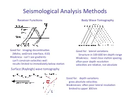
Receiver Functions Body Wave Tomography Surface Rayleigh wave tomography Good for Imaging discontinuities Moho sed rock interface 410 Weakness cant see gradients

Upload by phoebe-click
Published on 2016-07-10

Presentation Embed Code

<iframe width="560" height="315" src="https://www.docslides.com/embed/398243" frameborder="0" allowfullscreen></iframe>

Download Presentation

Download Presentation The PPT/PDF document "Seismological Analysis Methods" is the property of its rightful owner. Permission is granted to download and print the materials on this web site for personal, non-commercial use only, and to display it on your personal computer provided you do not modify the materials and that you retain all copyright notices contained in the materials. By downloading content from our website, you accept the terms of this agreement.