1 Lecture: Deep Networks Intro Topics: 1st lecture

slide1. 1 Lecture: Deep Networks Intro Topics: 1st lecture wrap-up, difficulty training deep networks,
image classification problem, using convolutions,
tricks to train deep networks


Resources: http://www.cs.utah.edu/~rajeev/cs7960/notes/
Canvas/registration<br>
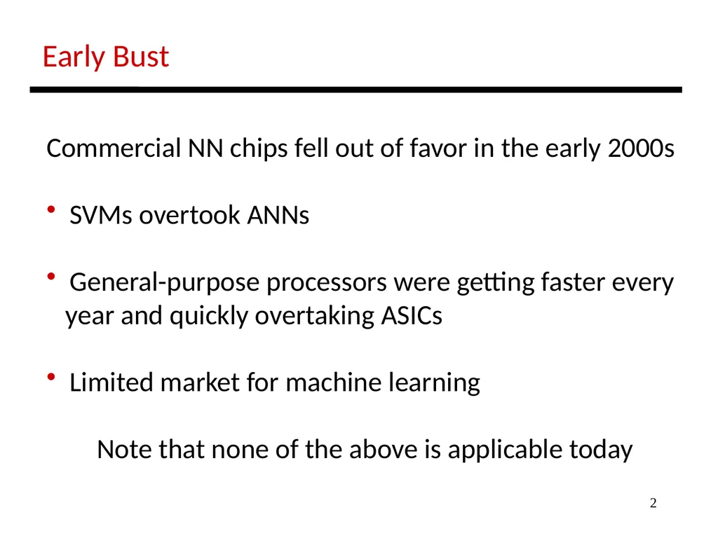
slide2. 2 Early Bust Commercial NN chips fell out of favor in the early 2000s

SVMs overtook ANNs

General-purpose processors were getting faster every
year and quickly overtaking ASICs

Limited market for machine learning

Note that none of the above is applicable today<br>
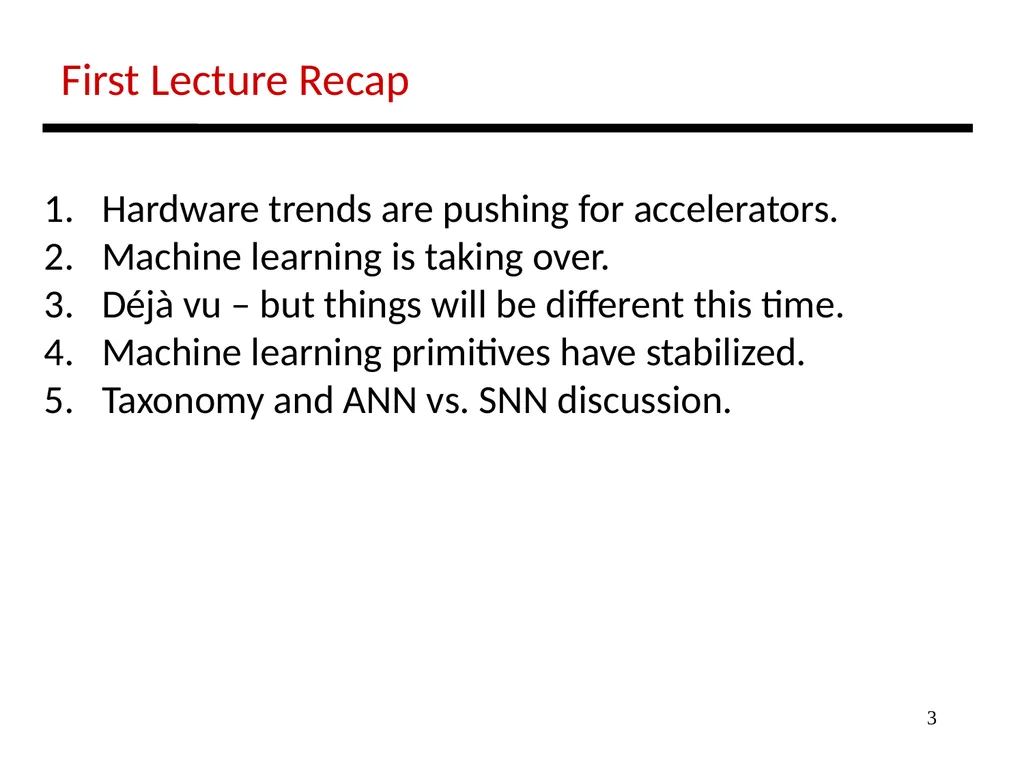
slide3. 3 First Lecture Recap Hardware trends are pushing for accelerators.
Machine learning is taking over.
Déjà vu – but things will be different this time.
Machine learning primitives have stabilized.
Taxonomy and ANN vs. SNN discussion.<br>
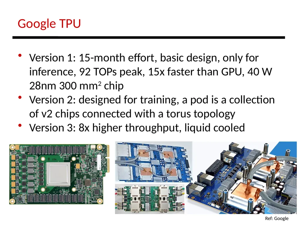
slide4. 4 Google TPU Version 1: 15-month effort, basic design, only for inference, 92 TOPs peak, 15x faster than GPU, 40 W 28nm 300 mm2 chip
Version 2: designed for training, a pod is a collection of v2 chips connected with a torus topology
Version 3: 8x higher throughput, liquid cooled Ref: Google<br>
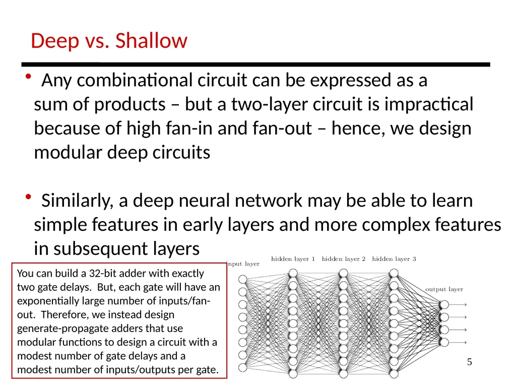
slide5. 5 Deep vs. Shallow Any combinational circuit can be expressed as a
sum of products – but a two-layer circuit is impractical
because of high fan-in and fan-out – hence, we design
modular deep circuits

Similarly, a deep neural network may be able to learn
simple features in early layers and more complex features
in subsequent layers You can build a 32-bit adder with exactly two gate delays. But, each gate will have an exponentially large number of inputs/fan-out. Therefore, we instead design generate-propagate adders that use modular functions to design a circuit with a modest number of gate delays and a modest number of inputs/outputs per gate.<br>
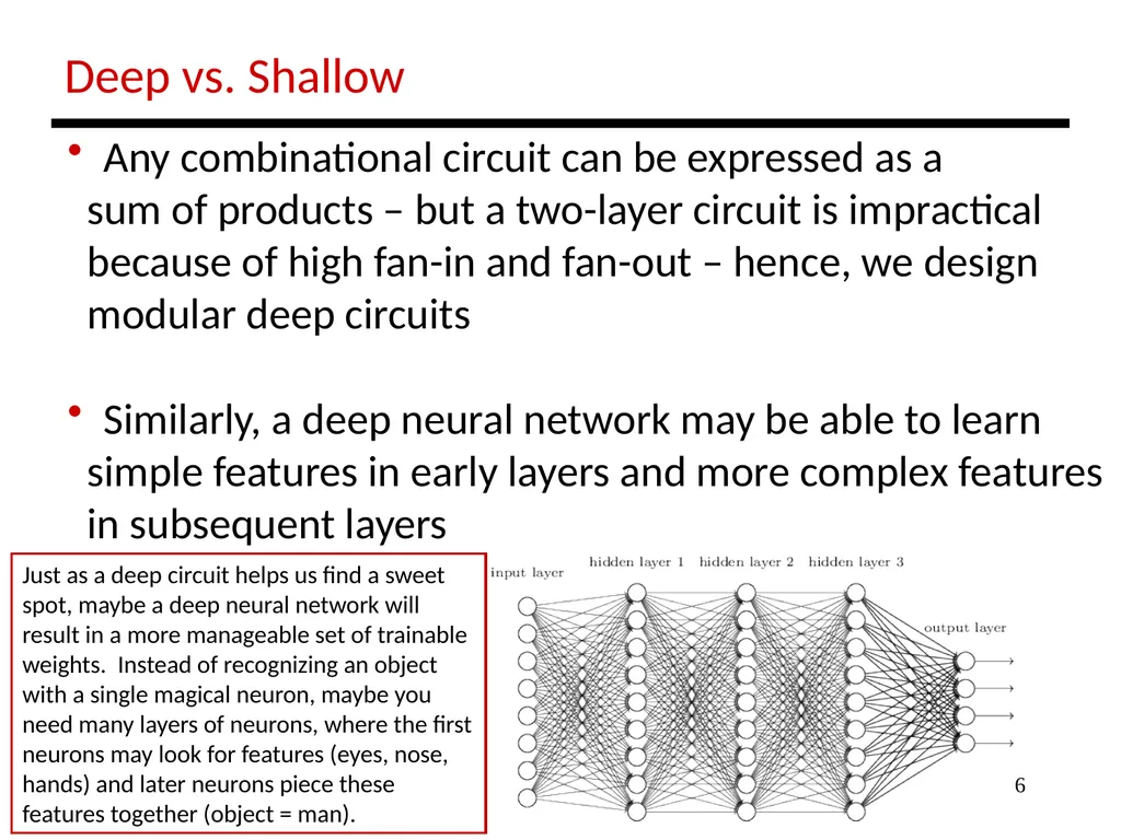
slide6. 6 Deep vs. Shallow Any combinational circuit can be expressed as a
sum of products – but a two-layer circuit is impractical
because of high fan-in and fan-out – hence, we design
modular deep circuits

Similarly, a deep neural network may be able to learn
simple features in early layers and more complex features
in subsequent layers Just as a deep circuit helps us find a sweet spot, maybe a deep neural network will result in a more manageable set of trainable weights. Instead of recognizing an object with a single magical neuron, maybe you need many layers of neurons, where the first neurons may look for features (eyes, nose, hands) and later neurons piece these features together (object = man).<br>
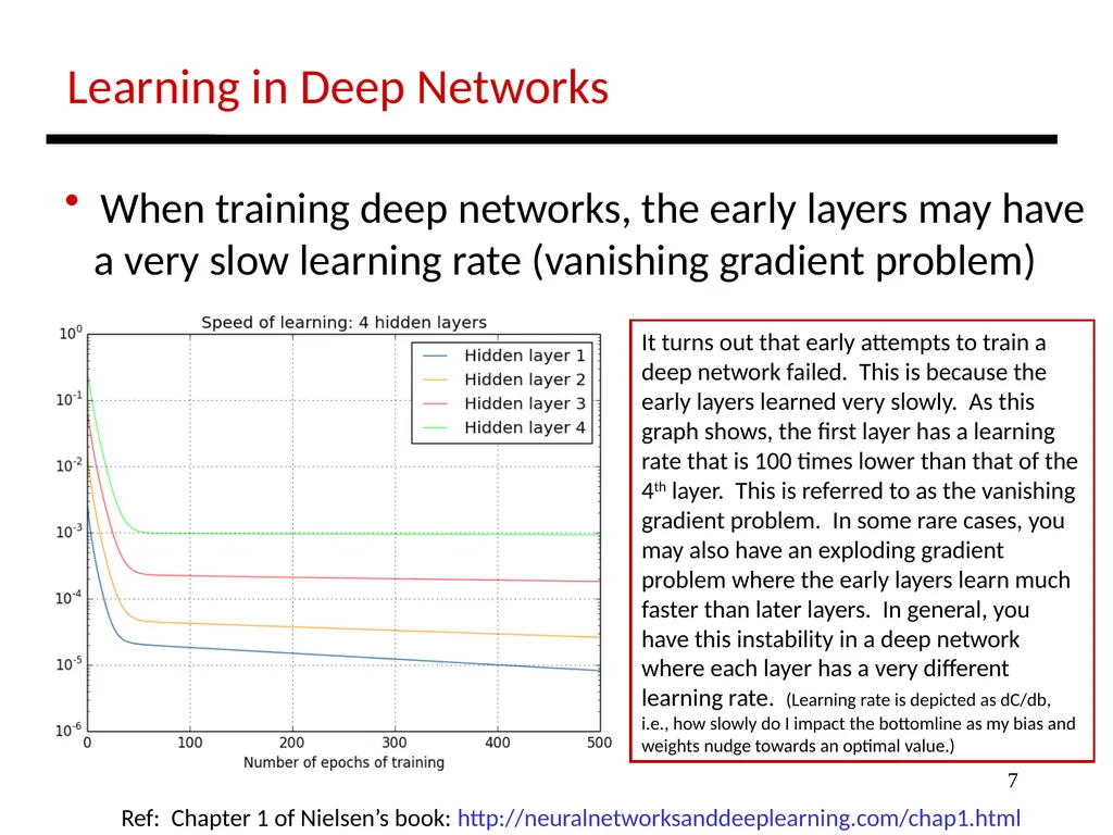
slide7. 7 Learning in Deep Networks When training deep networks, the early layers may have
a very slow learning rate (vanishing gradient problem) Ref: Chapter 1 of Nielsen’s book: http://neuralnetworksanddeeplearning.com/chap1.html It turns out that early attempts to train a deep network failed. This is because the early layers learned very slowly. As this graph shows, the first layer has a learning rate that is 100 times lower than that of the 4th layer. This is referred to as the vanishing gradient problem. In some rare cases, you may also have an exploding gradient problem where the early layers learn much faster than later layers. In general, you have this instability in a deep network where each layer has a very different learning rate. (Learning rate is depicted as dC/db, i.e., how slowly do I impact the bottomline as my bias and weights nudge towards an optimal value.)<br>
slide8. 8<br>
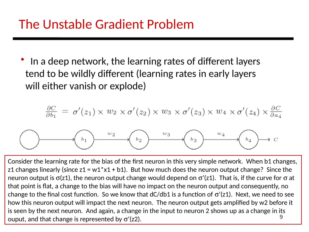
slide9. 9 The Unstable Gradient Problem In a deep network, the learning rates of different layers
tend to be wildly different (learning rates in early layers
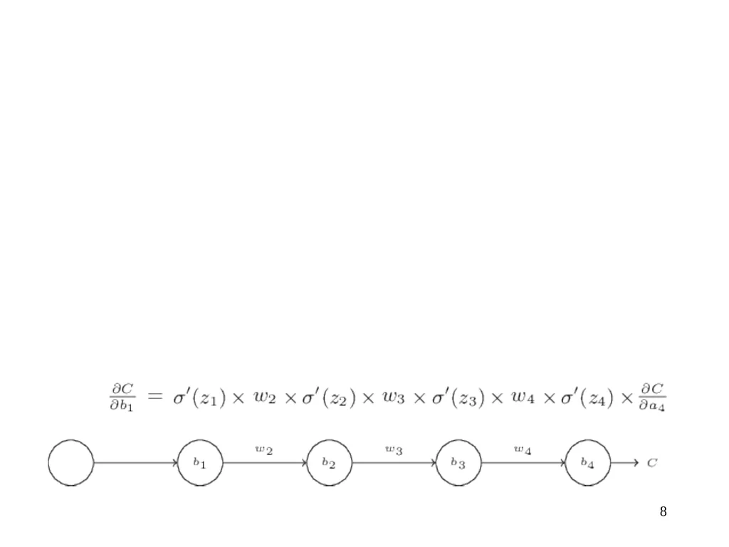
will either vanish or explode) Consider the learning rate for the bias of the first neuron in this very simple network. When b1 changes, z1 changes linearly (since z1 = w1*x1 + b1). But how much does the neuron output change? Since the neuron output is s(z1), the neuron output change would depend on s’(z1). That is, if the curve for s at that point is flat, a change to the bias will have no impact on the neuron output and consequently, no change to the final cost function. So we know that dC/db1 is a function of s’(z1). Next, we need to see how this neuron output will impact the next neuron. The neuron output gets amplified by w2 before it is seen by the next neuron. And again, a change in the input to neuron 2 shows up as a change in its ouput, and that change is represented by s’(z2).<br>
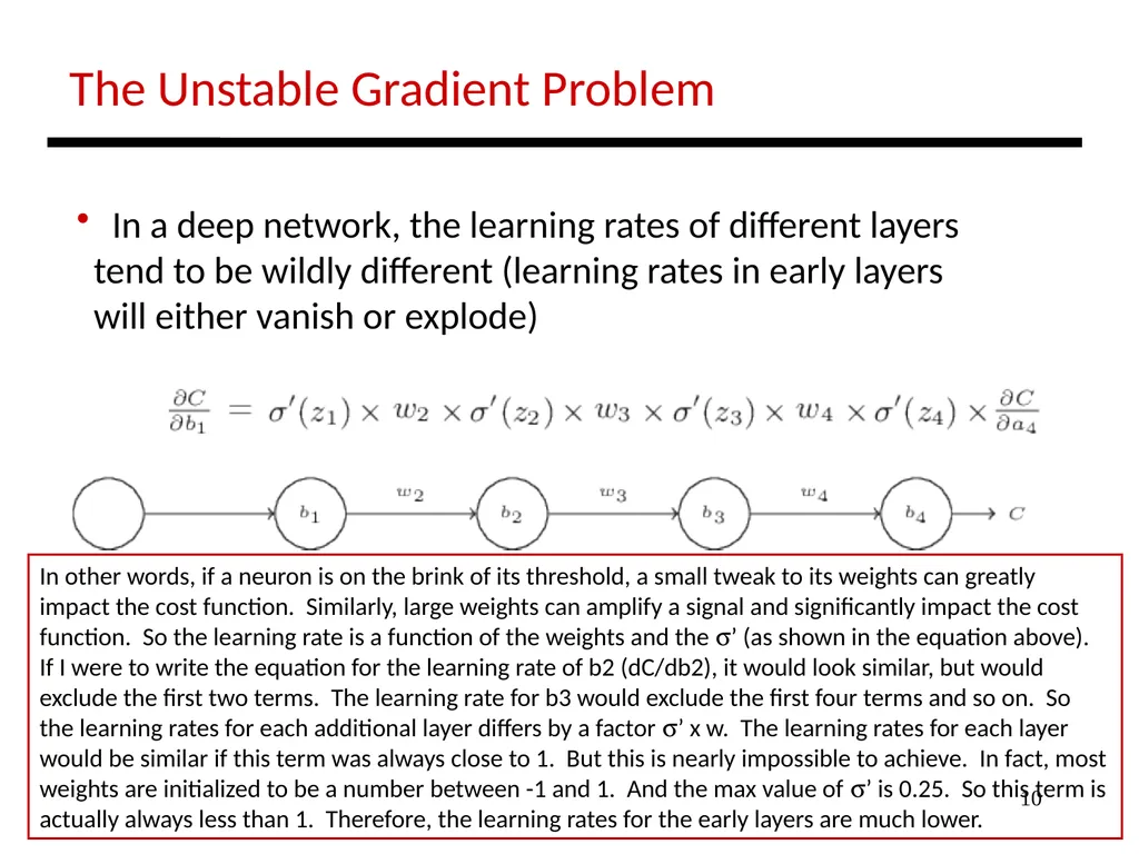
slide10. 10 The Unstable Gradient Problem In a deep network, the learning rates of different layers
tend to be wildly different (learning rates in early layers
will either vanish or explode) In other words, if a neuron is on the brink of its threshold, a small tweak to its weights can greatly impact the cost function. Similarly, large weights can amplify a signal and significantly impact the cost function. So the learning rate is a function of the weights and the s’ (as shown in the equation above).
If I were to write the equation for the learning rate of b2 (dC/db2), it would look similar, but would exclude the first two terms. The learning rate for b3 would exclude the first four terms and so on. So the learning rates for each additional layer differs by a factor s’ x w. The learning rates for each layer would be similar if this term was always close to 1. But this is nearly impossible to achieve. In fact, most weights are initialized to be a number between -1 and 1. And the max value of s’ is 0.25. So this term is actually always less than 1. Therefore, the learning rates for the early layers are much lower.<br>
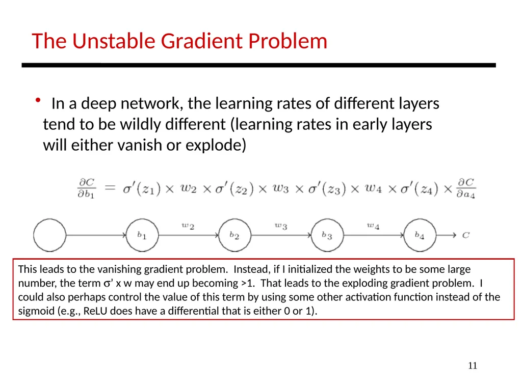
slide11. 11 The Unstable Gradient Problem In a deep network, the learning rates of different layers
tend to be wildly different (learning rates in early layers
will either vanish or explode) This leads to the vanishing gradient problem. Instead, if I initialized the weights to be some large number, the term s’ x w may end up becoming >1. That leads to the exploding gradient problem. I could also perhaps control the value of this term by using some other activation function instead of the sigmoid (e.g., ReLU does have a differential that is either 0 or 1).<br>
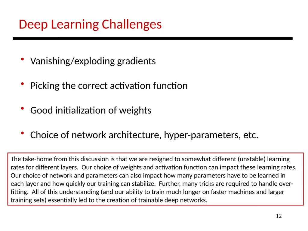
slide12. 12 Deep Learning Challenges Vanishing/exploding gradients

Picking the correct activation function

Good initialization of weights

Choice of network architecture, hyper-parameters, etc. The take-home from this discussion is that we are resigned to somewhat different (unstable) learning rates for different layers. Our choice of weights and activation function can impact these learning rates. Our choice of network and parameters can also impact how many parameters have to be learned in each layer and how quickly our training can stabilize. Further, many tricks are required to handle over-fitting. All of this understanding (and our ability to train much longer on faster machines and larger training sets) essentially led to the creation of trainable deep networks.<br>
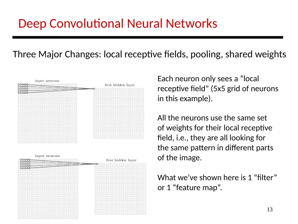
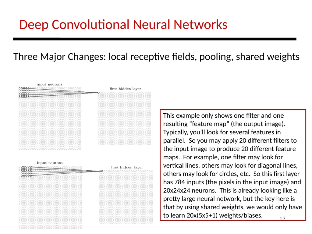
slide13. 13 Deep Convolutional Neural Networks Three Major Changes: local receptive fields, pooling, shared weights Each neuron only sees a “local
receptive field” (5x5 grid of neurons
in this example). All the neurons use the same set
of weights for their local receptive
field, i.e., they are all looking for
the same pattern in different parts
of the image.

What we’ve shown here is 1 “filter”
or 1 “feature map”.<br>
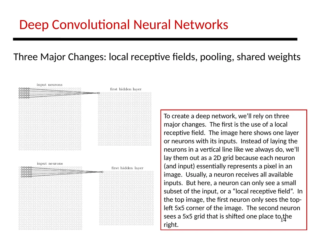
slide14. 14 Deep Convolutional Neural Networks Three Major Changes: local receptive fields, pooling, shared weights To create a deep network, we’ll rely on three major changes. The first is the use of a local receptive field. The image here shows one layer or neurons with its inputs. Instead of laying the neurons in a vertical line like we always do, we’ll lay them out as a 2D grid because each neuron (and input) essentially represents a pixel in an image. Usually, a neuron receives all available inputs. But here, a neuron can only see a small subset of the input, or a “local receptive field”. In the top image, the first neuron only sees the top-left 5x5 corner of the image. The second neuron sees a 5x5 grid that is shifted one place to the right.<br>
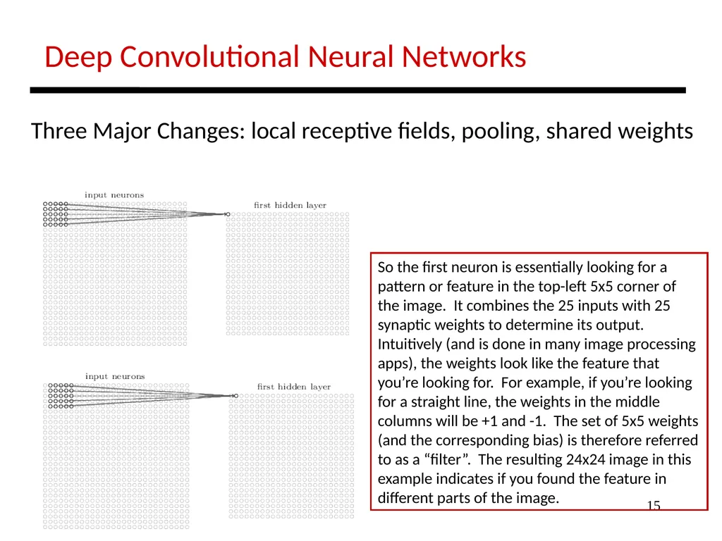
slide15. 15 Deep Convolutional Neural Networks Three Major Changes: local receptive fields, pooling, shared weights So the first neuron is essentially looking for a pattern or feature in the top-left 5x5 corner of the image. It combines the 25 inputs with 25 synaptic weights to determine its output. Intuitively (and is done in many image processing apps), the weights look like the feature that you’re looking for. For example, if you’re looking for a straight line, the weights in the middle columns will be +1 and -1. The set of 5x5 weights (and the corresponding bias) is therefore referred to as a “filter”. The resulting 24x24 image in this example indicates if you found the feature in different parts of the image.<br>
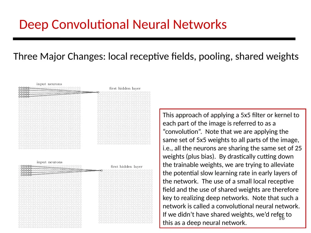
slide16. 16 Deep Convolutional Neural Networks Three Major Changes: local receptive fields, pooling, shared weights This approach of applying a 5x5 filter or kernel to each part of the image is referred to as a “convolution”. Note that we are applying the same set of 5x5 weights to all parts of the image, i.e., all the neurons are sharing the same set of 25 weights (plus bias). By drastically cutting down the trainable weights, we are trying to alleviate the potential slow learning rate in early layers of the network. The use of a small local receptive field and the use of shared weights are therefore key to realizing deep networks. Note that such a network is called a convolutional neural network. If we didn’t have shared weights, we’d refer to this as a deep neural network.<br>
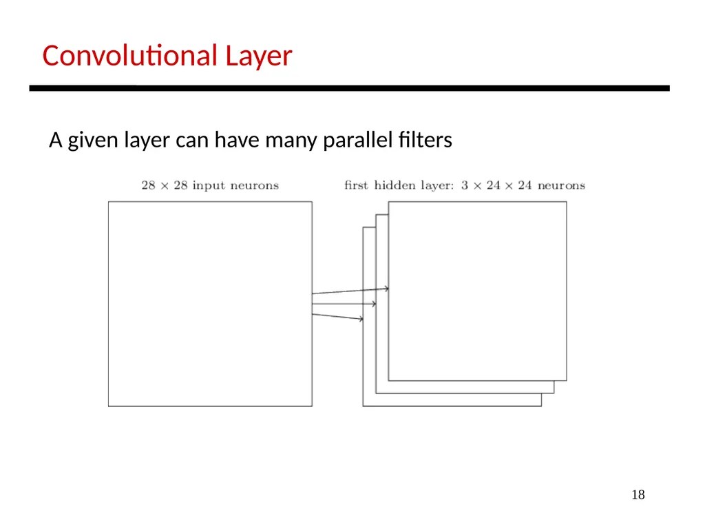
slide17. 17 Deep Convolutional Neural Networks Three Major Changes: local receptive fields, pooling, shared weights This example only shows one filter and one resulting “feature map” (the output image). Typically, you’ll look for several features in parallel. So you may apply 20 different filters to the input image to produce 20 different feature maps. For example, one filter may look for vertical lines, others may look for diagonal lines, others may look for circles, etc. So this first layer has 784 inputs (the pixels in the input image) and 20x24x24 neurons. This is already looking like a pretty large neural network, but the key here is that by using shared weights, we would only have to learn 20x(5x5+1) weights/biases.<br>
slide18. 18 Convolutional Layer A given layer can have many parallel filters<br>
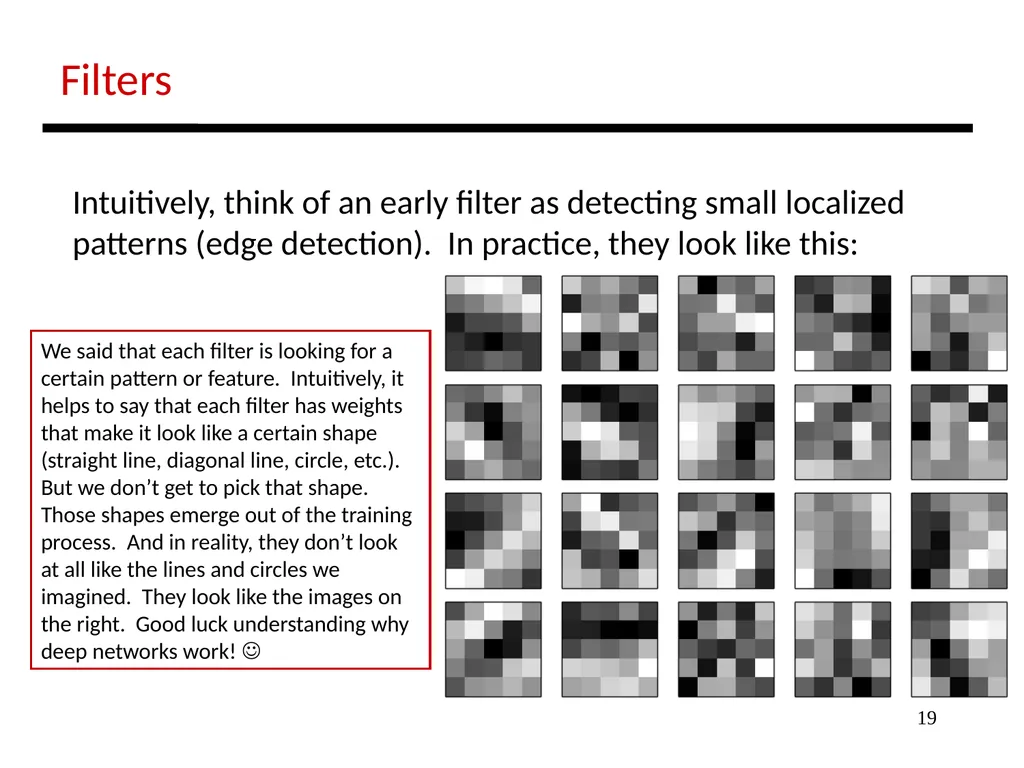
slide19. 19 Filters Intuitively, think of an early filter as detecting small localized
patterns (edge detection). In practice, they look like this: We said that each filter is looking for a certain pattern or feature. Intuitively, it helps to say that each filter has weights that make it look like a certain shape (straight line, diagonal line, circle, etc.). But we don’t get to pick that shape. Those shapes emerge out of the training process. And in reality, they don’t look at all like the lines and circles we imagined. They look like the images on the right. Good luck understanding why deep networks work! <br>
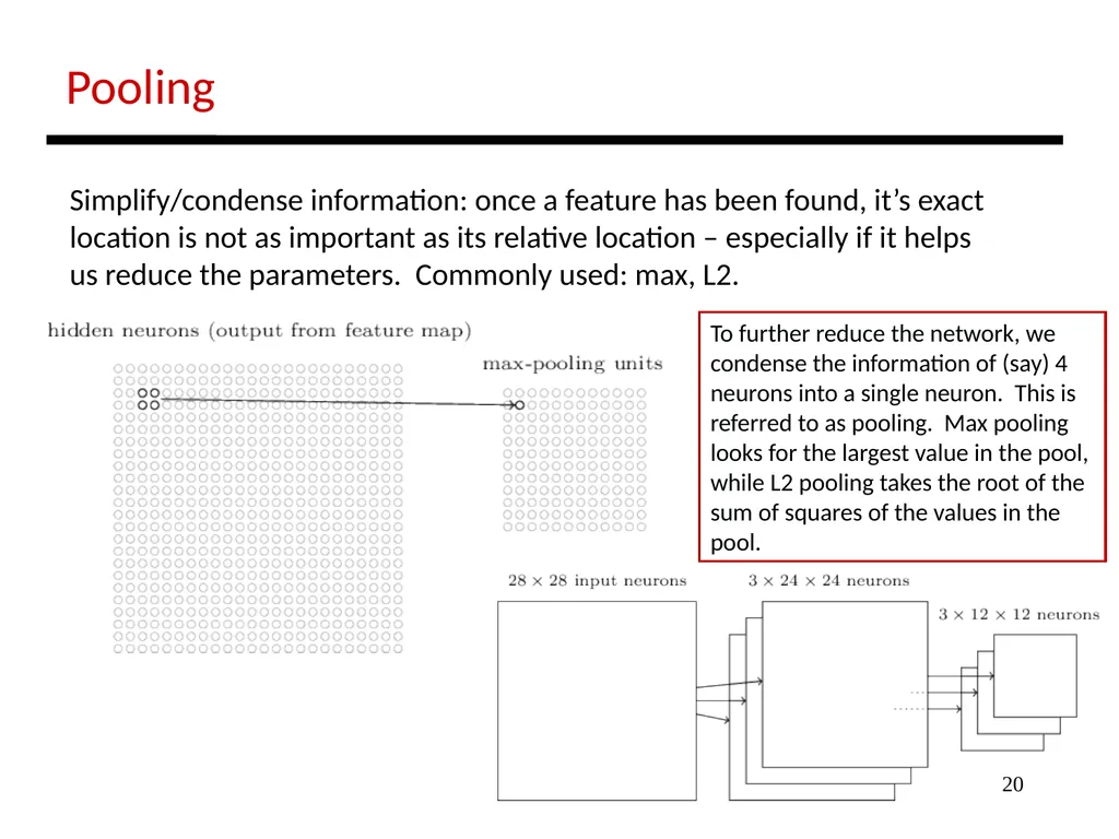
slide20. 20 Pooling Simplify/condense information: once a feature has been found, it’s exact
location is not as important as its relative location – especially if it helps
us reduce the parameters. Commonly used: max, L2. To further reduce the network, we condense the information of (say) 4 neurons into a single neuron. This is referred to as pooling. Max pooling looks for the largest value in the pool, while L2 pooling takes the root of the sum of squares of the values in the pool.<br>
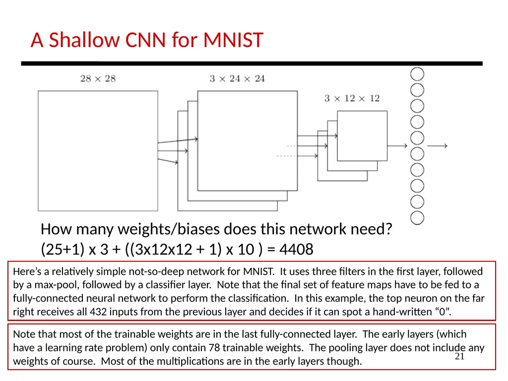
slide21. 21 A Shallow CNN for MNIST How many weights/biases does this network need?
(25+1) x 3 + ((3x12x12 + 1) x 10 ) = 4408 Here’s a relatively simple not-so-deep network for MNIST. It uses three filters in the first layer, followed by a max-pool, followed by a classifier layer. Note that the final set of feature maps have to be fed to a fully-connected neural network to perform the classification. In this example, the top neuron on the far right receives all 432 inputs from the previous layer and decides if it can spot a hand-written “0”. Note that most of the trainable weights are in the last fully-connected layer. The early layers (which have a learning rate problem) only contain 78 trainable weights. The pooling layer does not include any weights of course. Most of the multiplications are in the early layers though.<br>
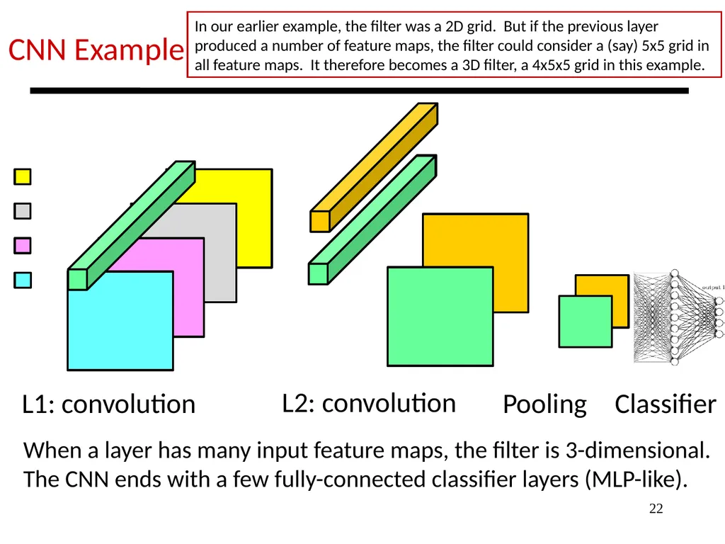
slide22. 22 CNN Example When a layer has many input feature maps, the filter is 3-dimensional.
The CNN ends with a few fully-connected classifier layers (MLP-like). L1: convolution L2: convolution Pooling Classifier In our earlier example, the filter was a 2D grid. But if the previous layer produced a number of feature maps, the filter could consider a (say) 5x5 grid in all feature maps. It therefore becomes a 3D filter, a 4x5x5 grid in this example.<br>
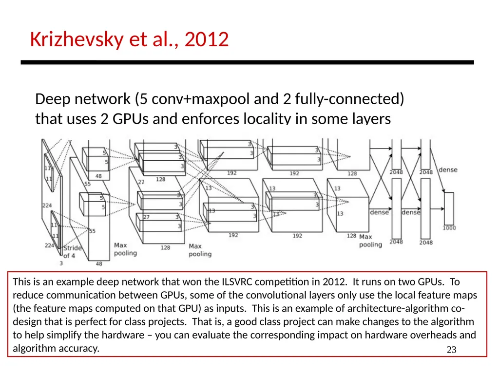
slide23. 23 Krizhevsky et al., 2012 Deep network (5 conv+maxpool and 2 fully-connected)
that uses 2 GPUs and enforces locality in some layers This is an example deep network that won the ILSVRC competition in 2012. It runs on two GPUs. To reduce communication between GPUs, some of the convolutional layers only use the local feature maps (the feature maps computed on that GPU) as inputs. This is an example of architecture-algorithm co-design that is perfect for class projects. That is, a good class project can make changes to the algorithm to help simplify the hardware – you can evaluate the corresponding impact on hardware overheads and algorithm accuracy.<br>
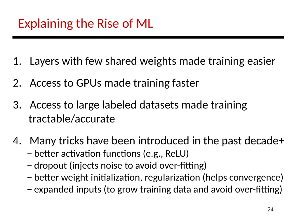
slide24. 24 Explaining the Rise of ML Layers with few shared weights made training easier

Access to GPUs made training faster

Access to large labeled datasets made training
tractable/accurate

4. Many tricks have been introduced in the past decade+
better activation functions (e.g., ReLU)
dropout (injects noise to avoid over-fitting)
better weight initialization, regularization (helps convergence)
expanded inputs (to grow training data and avoid over-fitting)<br>
slide25. 25 References Chapters 5 and 6 of Nielsen’s book:
http://neuralnetworksanddeeplearning.com<br>