
CS344: Introduction to Artificial Intelligence



Description: CS344: Introduction to Artificial Intelligence (associated lab: CS386) Pushpak Bhattacharyya CSE Dept., IIT Bombay Lecture 34: Backpropagation; need for multiple layers and non linearity 5th April, 2011 Backpropagation algorithm Fully
Related Topics
Download Presentation
"CS344: Introduction to Artificial Intelligence" is the property of its rightful owner. Permission is granted to download and print the materials on this website for personal, non-commercial use only, and to display it on your personal computer provided you do not modify the materials and that you retain all copyright notices contained in the materials. By downloading content from our website, you accept the terms of this agreement.
Presentation Transcript
slide1. CS344: Introduction to Artificial Intelligence
(associated lab: CS386) Pushpak Bhattacharyya
CSE Dept.,
IIT Bombay
Lecture 34: Backpropagation; need for multiple layers and non linearity
5th April, 2011<br>
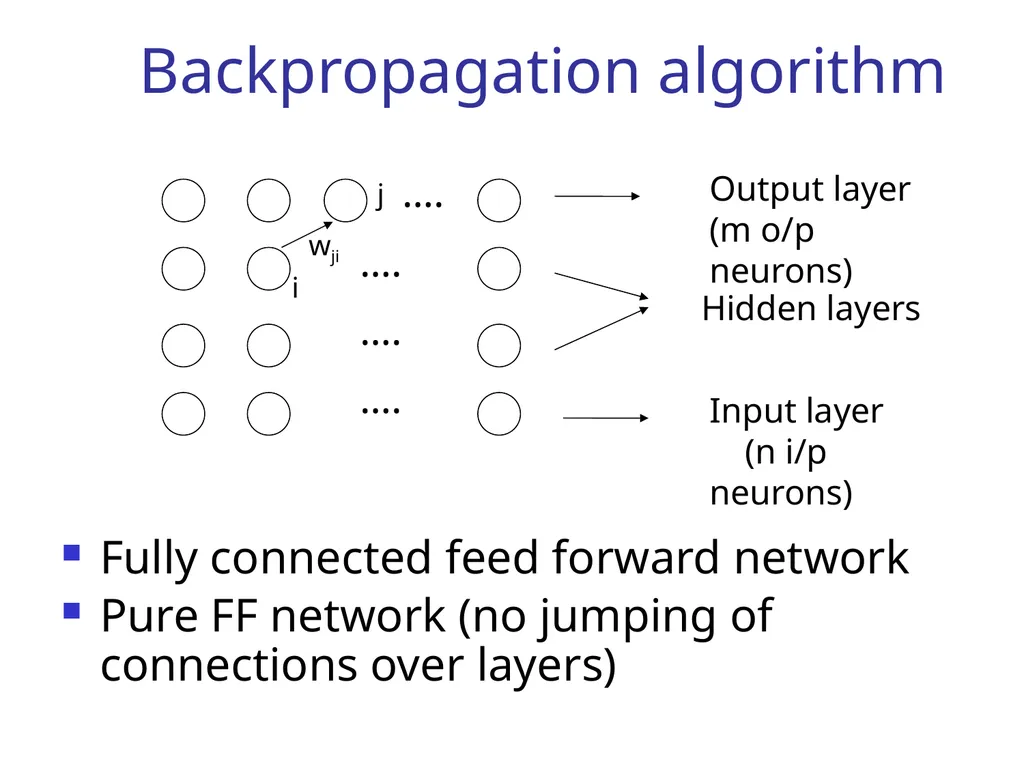
slide2. Backpropagation algorithm Fully connected feed forward network
Pure FF network (no jumping of connections over layers) Hidden layers Input layer (n i/p neurons) Output layer (m o/p neurons) j i wji …. …. …. ….<br>
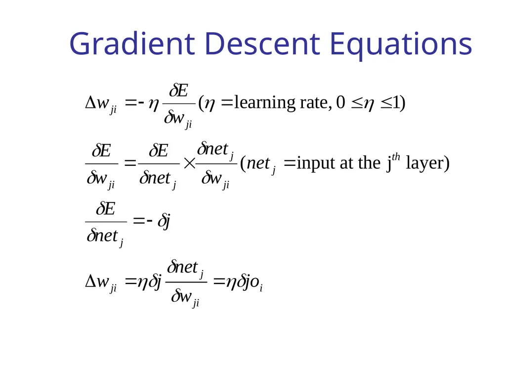
slide3. Gradient Descent Equations<br>
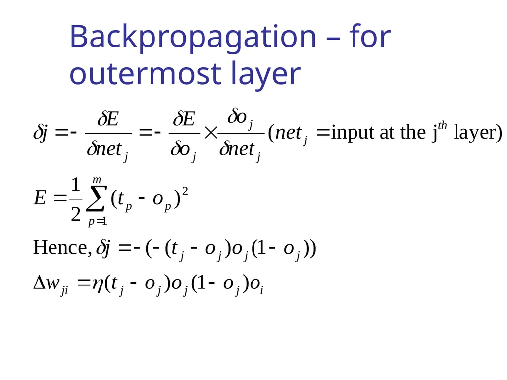
slide4. Backpropagation – for outermost layer<br>
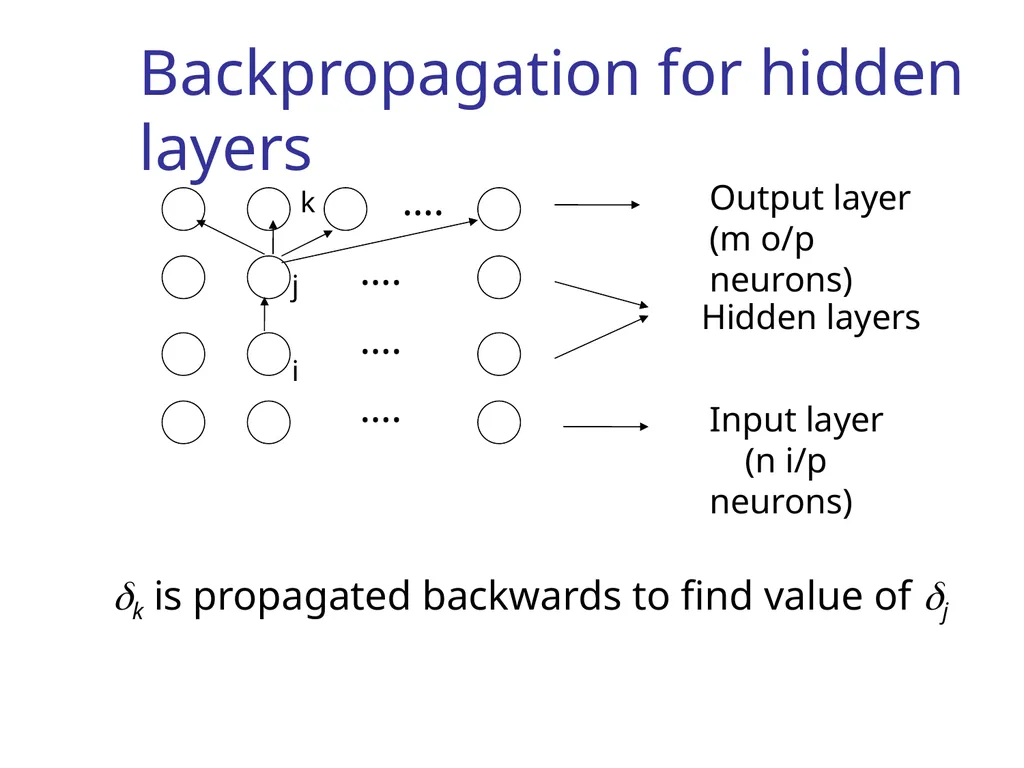
slide5. Backpropagation for hidden layers Hidden layers Input layer (n i/p neurons) Output layer (m o/p neurons) j i …. …. …. …. k k is propagated backwards to find value of j<br>
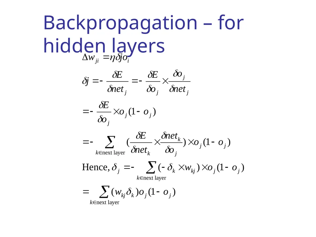
slide6. Backpropagation – for hidden layers<br>
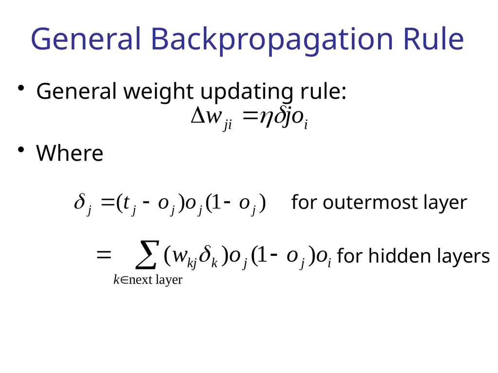
slide7. General Backpropagation Rule General weight updating rule:
Where for outermost layer for hidden layers<br>
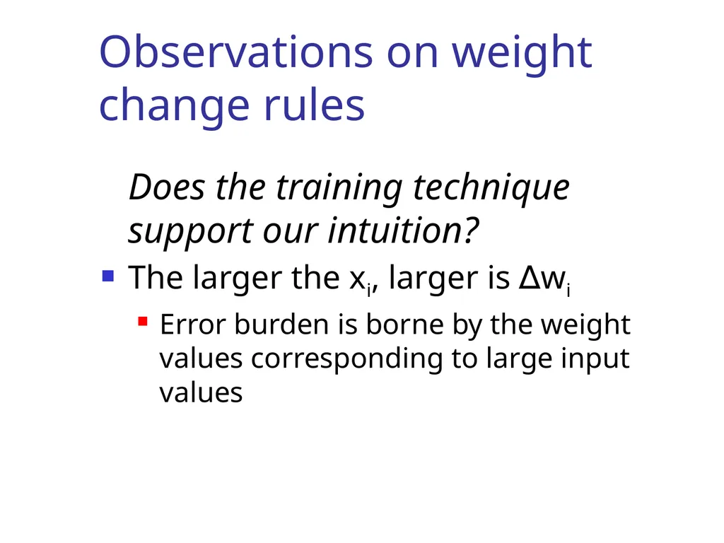
slide8. Observations on weight change rules Does the training technique support our intuition?
The larger the xi, larger is ∆wi
Error burden is borne by the weight values corresponding to large input values<br>
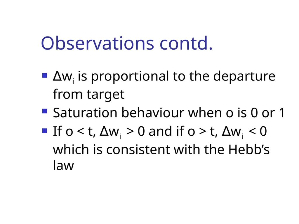
slide9. Observations contd. ∆wi is proportional to the departure from target
Saturation behaviour when o is 0 or 1
If o < t, ∆wi > 0 and if o > t, ∆wi < 0 which is consistent with the Hebb’s law<br>
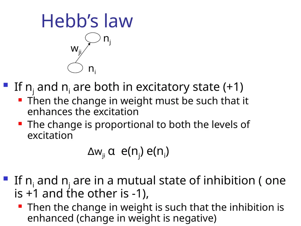
slide10. Hebb’s law If nj and ni are both in excitatory state (+1)
Then the change in weight must be such that it enhances the excitation
The change is proportional to both the levels of excitation
∆wji α e(nj) e(ni)
If ni and nj are in a mutual state of inhibition ( one is +1 and the other is -1),
Then the change in weight is such that the inhibition is enhanced (change in weight is negative) nj ni wji<br>
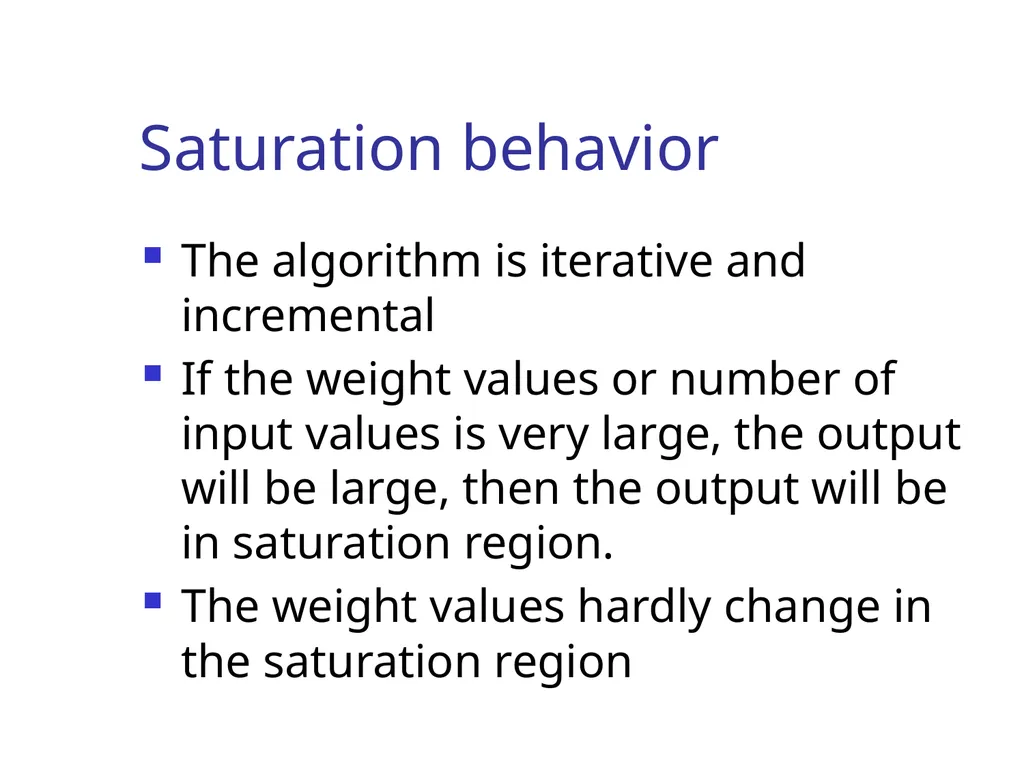
slide11. Saturation behavior The algorithm is iterative and incremental
If the weight values or number of input values is very large, the output will be large, then the output will be in saturation region.
The weight values hardly change in the saturation region<br>
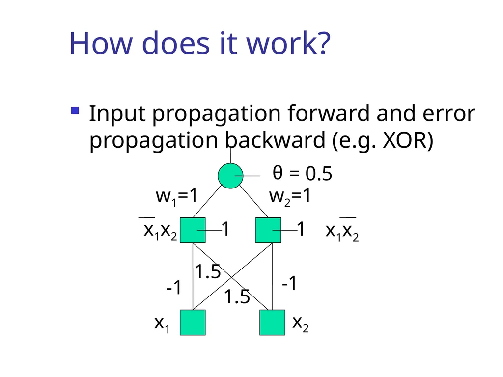
slide12. How does it work? Input propagation forward and error propagation backward (e.g. XOR)<br>
slide13. If Sigmoid Neurons Are Used, Do We Need MLP?
Does sigmoid have the power of separating non-linearly separable data?
Can sigmoid solve the X-OR problem<br>
slide14. O = 1 if O > yu
O = 0 if O < yl
Typically yl << 0.5 , yu >> 0.5 O = 1 / 1+ e -net O net 1 yu yl<br>
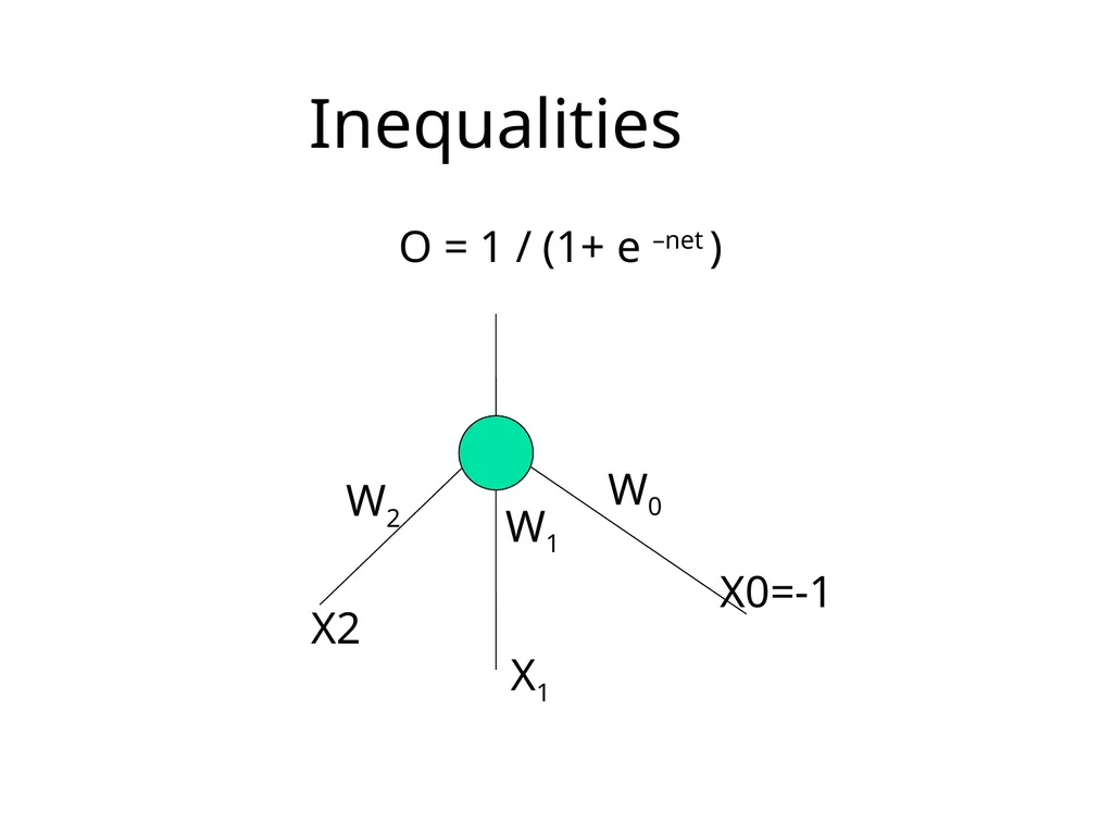
slide15. Inequalities O = 1 / (1+ e –net )<br>
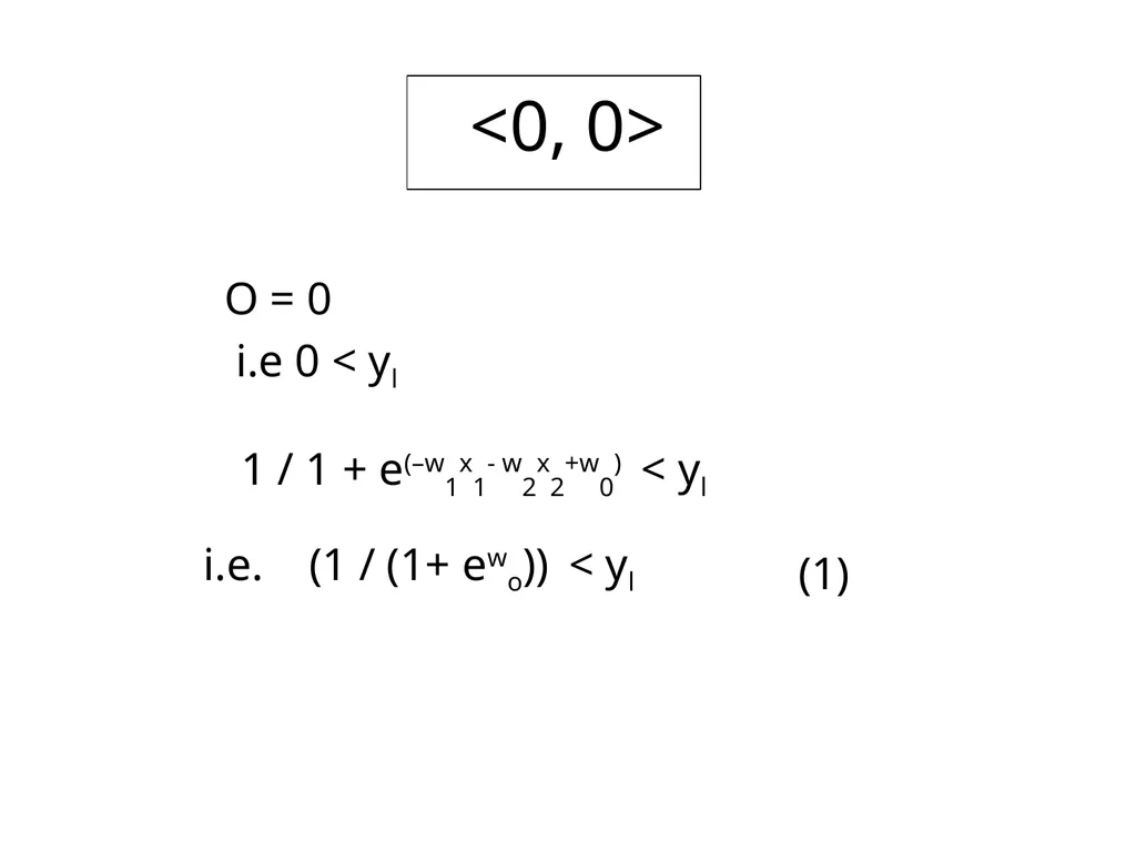
slide16. <0, 0>
O = 0
i.e 0 < yl 1 / 1 + e(–w1x1- w2x2+w0) < yl i.e. (1 / (1+ ewo)) < yl (1)<br>
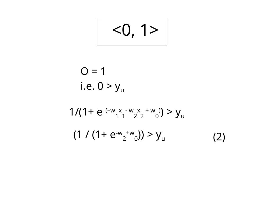
slide17. <0, 1>
O = 1
i.e. 0 > yu 1/(1+ e (–w1x1- w2x2 + w0)) > yu (1 / (1+ e-w2+w0)) > yu (2)<br>
slide18. <1, 0>
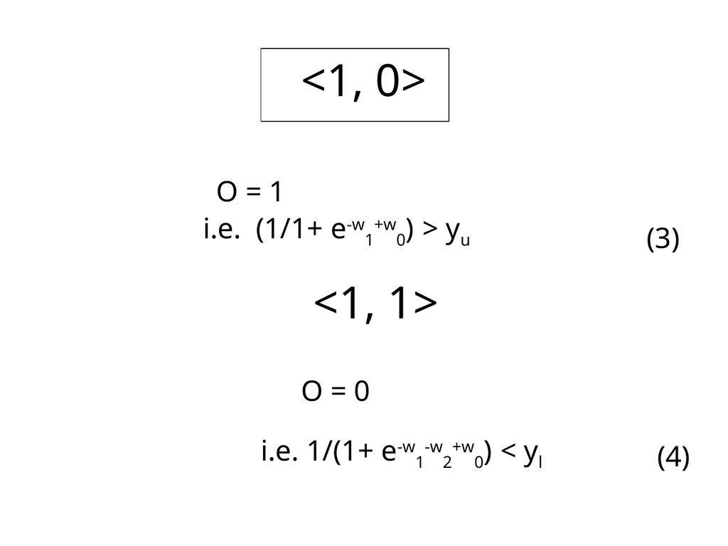
O = 1 i.e. (1/1+ e-w1+w0) > yu <1, 1>
O = 0 i.e. 1/(1+ e-w1-w2+w0) < yl (3) (4)<br>
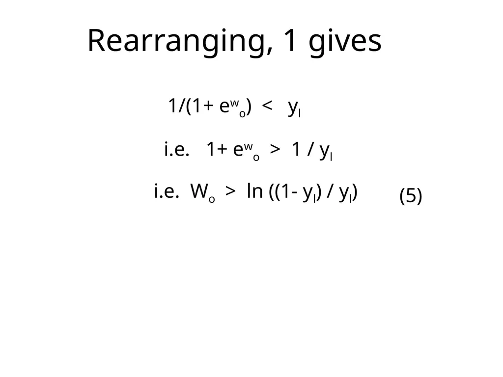
slide19. Rearranging, 1 gives i.e. 1+ ewo > 1 / yl i.e. Wo > ln ((1- yl) / yl) (5) 1/(1+ ewo) < yl<br>
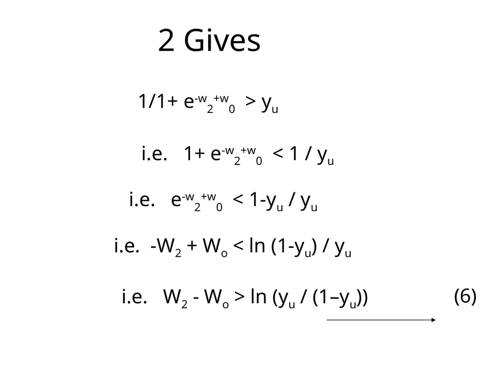
slide20. 2 Gives 1/1+ e-w2+w0 > yu i.e. 1+ e-w2+w0 < 1 / yu i.e. e-w2+w0 < 1-yu / yu i.e. -W2 + Wo < ln (1-yu) / yu i.e. W2 - Wo > ln (yu / (1–yu)) (6)<br>
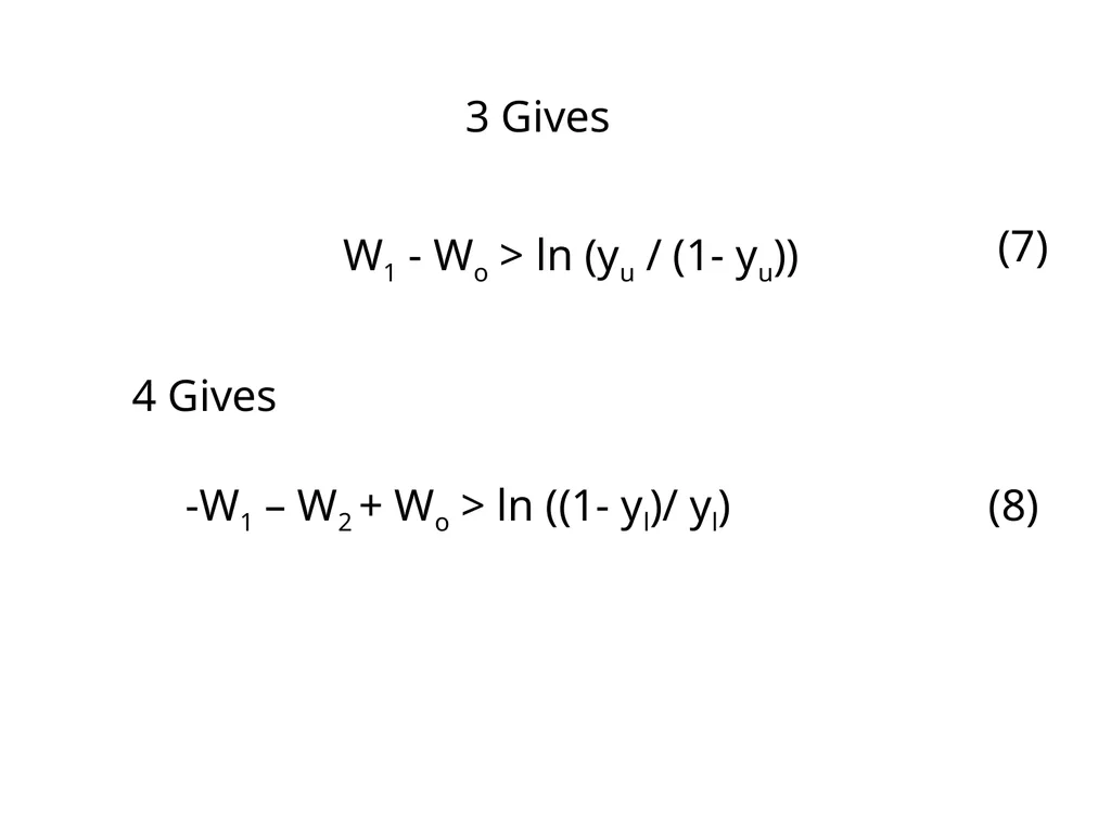
slide21. W1 - Wo > ln (yu / (1- yu)) -W1 – W2 + Wo > ln ((1- yl)/ yl) 3 Gives 4 Gives (7) (8)<br>
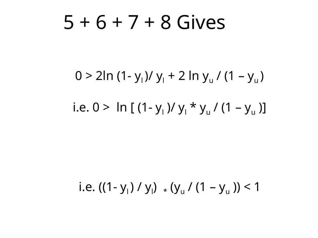
slide22. 5 + 6 + 7 + 8 Gives 0 > 2ln (1- yl )/ yl + 2 ln yu / (1 – yu )
i.e. 0 > ln [ (1- yl )/ yl * yu / (1 – yu )] i.e. ((1- yl ) / yl) * (yu / (1 – yu )) < 1<br>
slide23. [(1- yl ) / (1- yy )] * [yu / yl] < 1
2) Yu >> 0.5
3) Yl << 0.5
From i, ii and iii; Contradiction, hence sigmoid cannot compute X-OR<br>
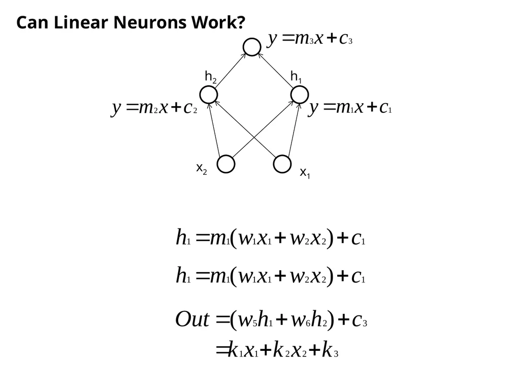
slide24. x2 x1 h2 h1 Can Linear Neurons Work?<br>
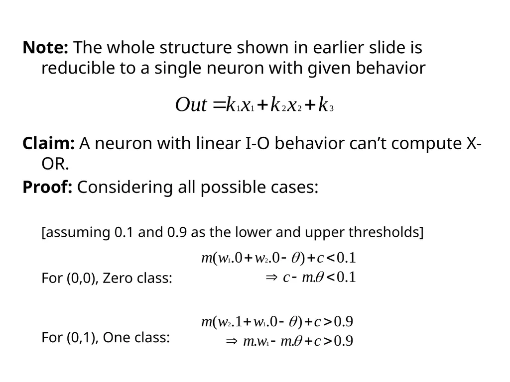
slide25. Note: The whole structure shown in earlier slide is reducible to a single neuron with given behavior
Claim: A neuron with linear I-O behavior can’t compute X-OR.
Proof: Considering all possible cases:
[assuming 0.1 and 0.9 as the lower and upper thresholds]
For (0,0), Zero class:
For (0,1), One class:<br>
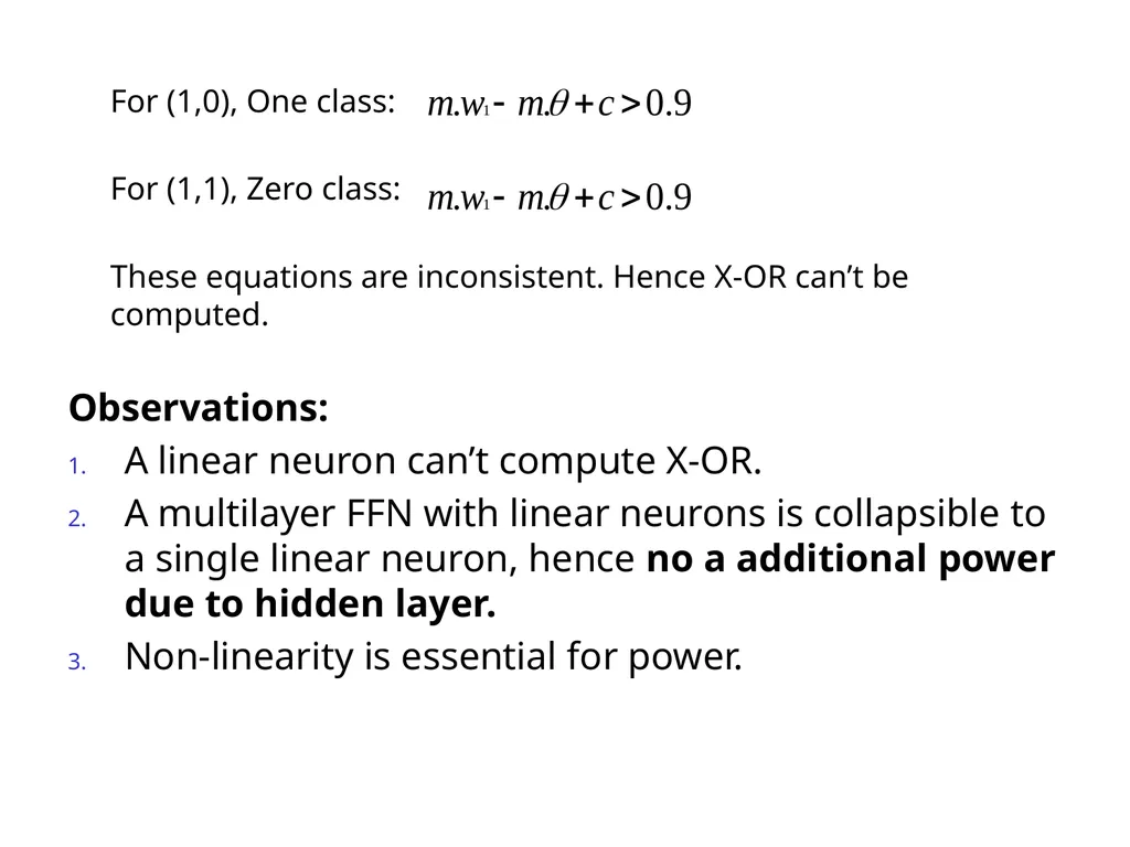
slide26. For (1,0), One class:
For (1,1), Zero class:
These equations are inconsistent. Hence X-OR can’t be computed.
Observations:
A linear neuron can’t compute X-OR.
A multilayer FFN with linear neurons is collapsible to a single linear neuron, hence no a additional power due to hidden layer.
Non-linearity is essential for power.<br>
Lecture 34: Backpropagation; need for multiple layers and non linearity
5th April, 2011<br>
slide2. Backpropagation algorithm Fully connected feed forward network
Pure FF network (no jumping of connections over layers) Hidden layers Input layer (n i/p neurons) Output layer (m o/p neurons) j i wji …. …. …. ….<br>
slide3. Gradient Descent Equations<br>
slide4. Backpropagation – for outermost layer<br>
slide5. Backpropagation for hidden layers Hidden layers Input layer (n i/p neurons) Output layer (m o/p neurons) j i …. …. …. …. k k is propagated backwards to find value of j<br>
slide6. Backpropagation – for hidden layers<br>
slide7. General Backpropagation Rule General weight updating rule:
Where for outermost layer for hidden layers<br>
slide8. Observations on weight change rules Does the training technique support our intuition?
The larger the xi, larger is ∆wi
Error burden is borne by the weight values corresponding to large input values<br>
slide9. Observations contd. ∆wi is proportional to the departure from target
Saturation behaviour when o is 0 or 1
If o < t, ∆wi > 0 and if o > t, ∆wi < 0 which is consistent with the Hebb’s law<br>
slide10. Hebb’s law If nj and ni are both in excitatory state (+1)
Then the change in weight must be such that it enhances the excitation
The change is proportional to both the levels of excitation
∆wji α e(nj) e(ni)
If ni and nj are in a mutual state of inhibition ( one is +1 and the other is -1),
Then the change in weight is such that the inhibition is enhanced (change in weight is negative) nj ni wji<br>
slide11. Saturation behavior The algorithm is iterative and incremental
If the weight values or number of input values is very large, the output will be large, then the output will be in saturation region.
The weight values hardly change in the saturation region<br>
slide12. How does it work? Input propagation forward and error propagation backward (e.g. XOR)<br>
slide13. If Sigmoid Neurons Are Used, Do We Need MLP?
Does sigmoid have the power of separating non-linearly separable data?
Can sigmoid solve the X-OR problem<br>
slide14. O = 1 if O > yu
O = 0 if O < yl
Typically yl << 0.5 , yu >> 0.5 O = 1 / 1+ e -net O net 1 yu yl<br>
slide15. Inequalities O = 1 / (1+ e –net )<br>
slide16. <0, 0>
O = 0
i.e 0 < yl 1 / 1 + e(–w1x1- w2x2+w0) < yl i.e. (1 / (1+ ewo)) < yl (1)<br>
slide17. <0, 1>
O = 1
i.e. 0 > yu 1/(1+ e (–w1x1- w2x2 + w0)) > yu (1 / (1+ e-w2+w0)) > yu (2)<br>
slide18. <1, 0>
O = 1 i.e. (1/1+ e-w1+w0) > yu <1, 1>
O = 0 i.e. 1/(1+ e-w1-w2+w0) < yl (3) (4)<br>
slide19. Rearranging, 1 gives i.e. 1+ ewo > 1 / yl i.e. Wo > ln ((1- yl) / yl) (5) 1/(1+ ewo) < yl<br>
slide20. 2 Gives 1/1+ e-w2+w0 > yu i.e. 1+ e-w2+w0 < 1 / yu i.e. e-w2+w0 < 1-yu / yu i.e. -W2 + Wo < ln (1-yu) / yu i.e. W2 - Wo > ln (yu / (1–yu)) (6)<br>
slide21. W1 - Wo > ln (yu / (1- yu)) -W1 – W2 + Wo > ln ((1- yl)/ yl) 3 Gives 4 Gives (7) (8)<br>
slide22. 5 + 6 + 7 + 8 Gives 0 > 2ln (1- yl )/ yl + 2 ln yu / (1 – yu )
i.e. 0 > ln [ (1- yl )/ yl * yu / (1 – yu )] i.e. ((1- yl ) / yl) * (yu / (1 – yu )) < 1<br>
slide23. [(1- yl ) / (1- yy )] * [yu / yl] < 1
2) Yu >> 0.5
3) Yl << 0.5
From i, ii and iii; Contradiction, hence sigmoid cannot compute X-OR<br>
slide24. x2 x1 h2 h1 Can Linear Neurons Work?<br>
slide25. Note: The whole structure shown in earlier slide is reducible to a single neuron with given behavior
Claim: A neuron with linear I-O behavior can’t compute X-OR.
Proof: Considering all possible cases:
[assuming 0.1 and 0.9 as the lower and upper thresholds]
For (0,0), Zero class:
For (0,1), One class:<br>
slide26. For (1,0), One class:
For (1,1), Zero class:
These equations are inconsistent. Hence X-OR can’t be computed.
Observations:
A linear neuron can’t compute X-OR.
A multilayer FFN with linear neurons is collapsible to a single linear neuron, hence no a additional power due to hidden layer.
Non-linearity is essential for power.<br>