Growth curve analysis What do those numbers mean?

slide1. Growth curve analysis What do those numbers mean?

Matt Winn (this presentation works best when you view it as a presentation, and not just the slides in editor view)<br>
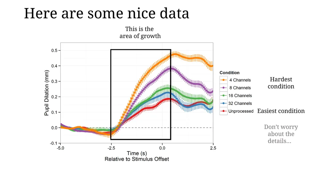
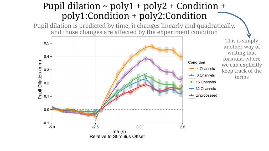
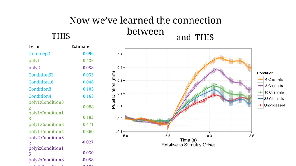
slide2. Here are some nice data This is the area of growth Hardest condition Easiest condition Don’t worry about the details…<br>
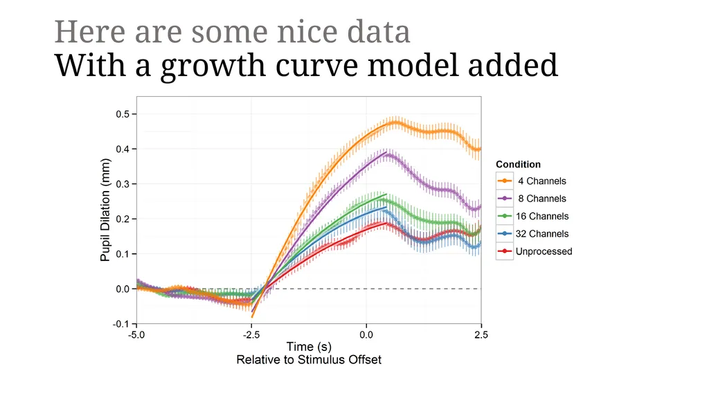
slide3. Here are some nice data
With a growth curve model added<br>
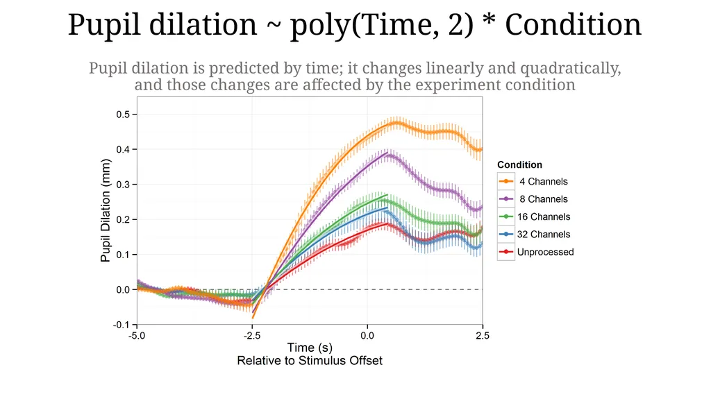
slide4. Pupil dilation ~ poly(Time, 2) * Condition Pupil dilation is predicted by time; it changes linearly and quadratically,
and those changes are affected by the experiment condition<br>
slide5. Pupil dilation ~ poly1 + poly2 + Condition +poly1:Condition + poly2:Condition Pupil dilation is predicted by time; it changes linearly and quadratically,
and those changes are affected by the experiment condition This is simply another way of writing that formula, where we can explicitly keep track of the terms<br>
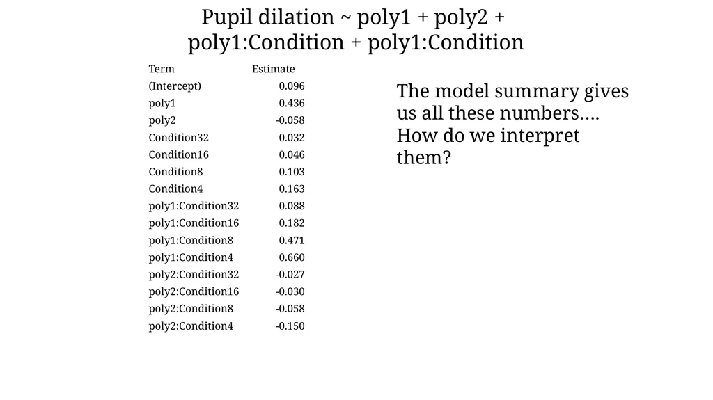
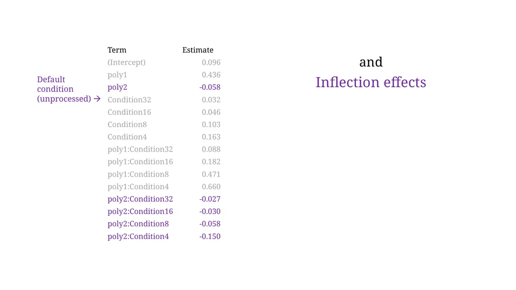
slide6. The model summary gives us all these numbers….
How do we interpret them? Pupil dilation ~ poly1 + poly2 + poly1:Condition + poly1:Condition<br>
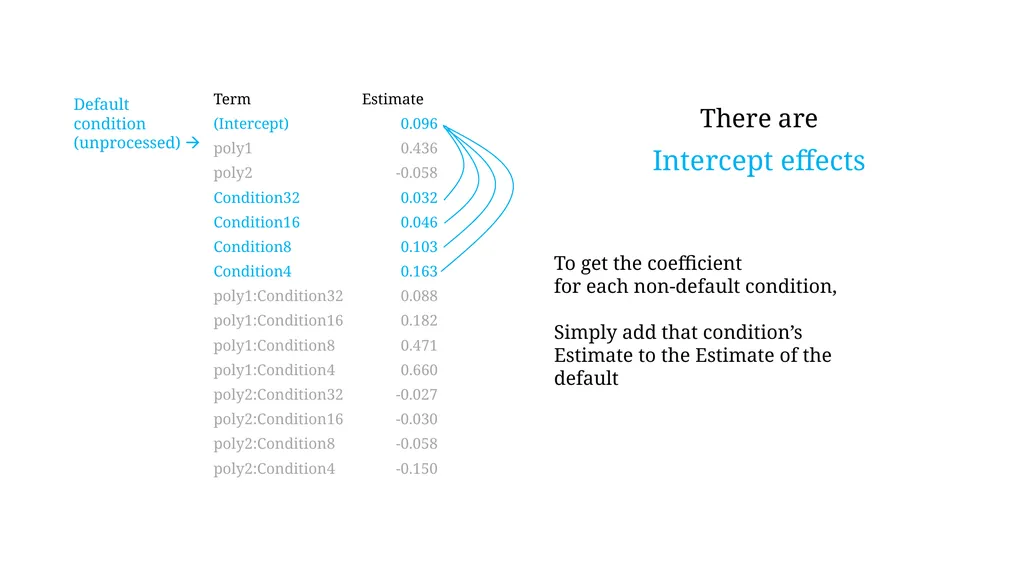
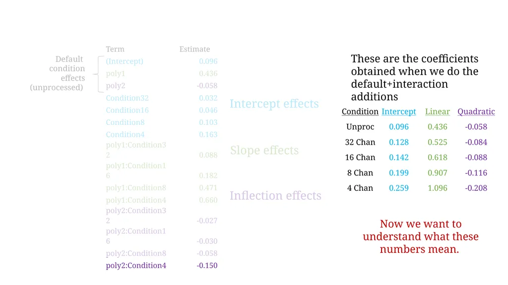
slide7. Intercept effects Default condition(unprocessed)  There are To get the coefficient for each non-default condition,
Simply add that condition’s Estimate to the Estimate of the default<br>
slide8. Slope effects Default condition(unprocessed)  and<br>
slide9. Inflection effects Default condition(unprocessed)  and<br>
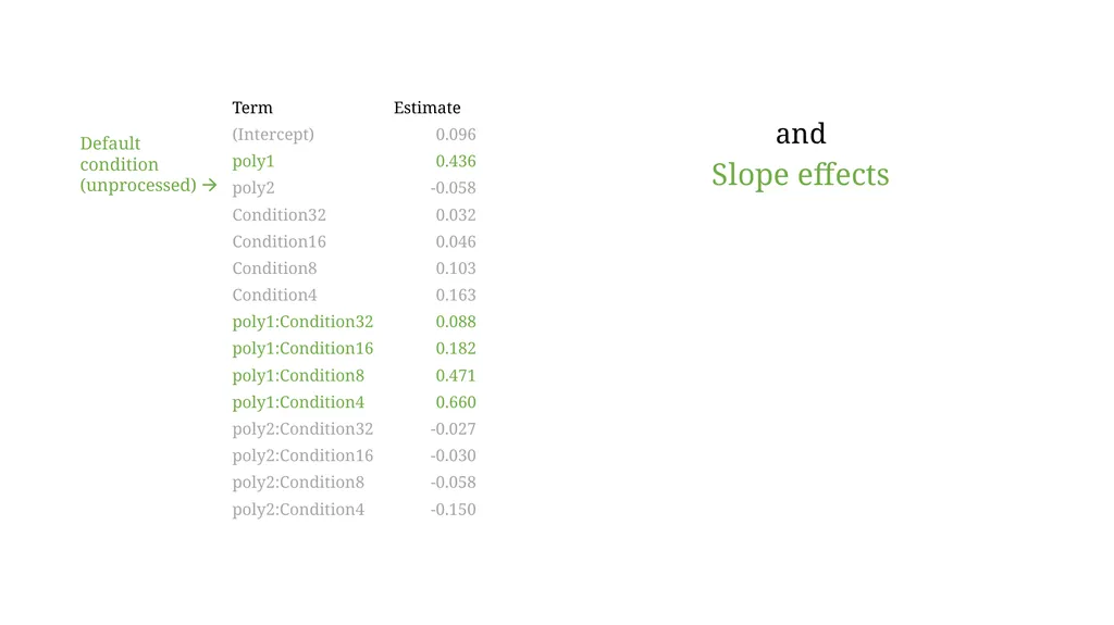
slide10. Inflection effects Default condition
effects(unprocessed) Slope effects Intercept effects These are the coefficients obtained when we do the default+interaction additions Now we want to understand what these numbers mean.<br>
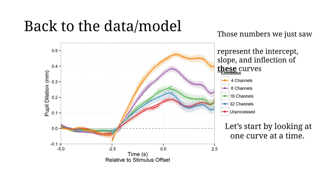
slide11. Back to the data/model Those numbers we just saw represent the intercept, slope, and inflection of these curves Let’s start by looking at one curve at a time.<br>
slide12. Now let’s take a look at the individual components Components:

Slope

Inflection<br>
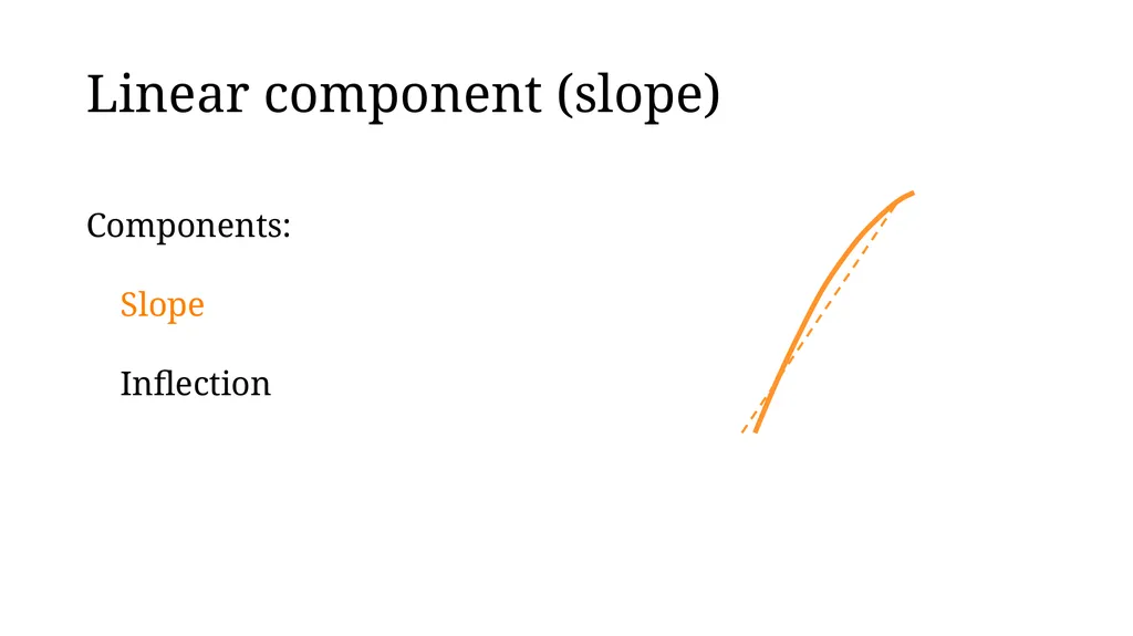
slide13. Linear component (slope) Components:

Slope

Inflection<br>
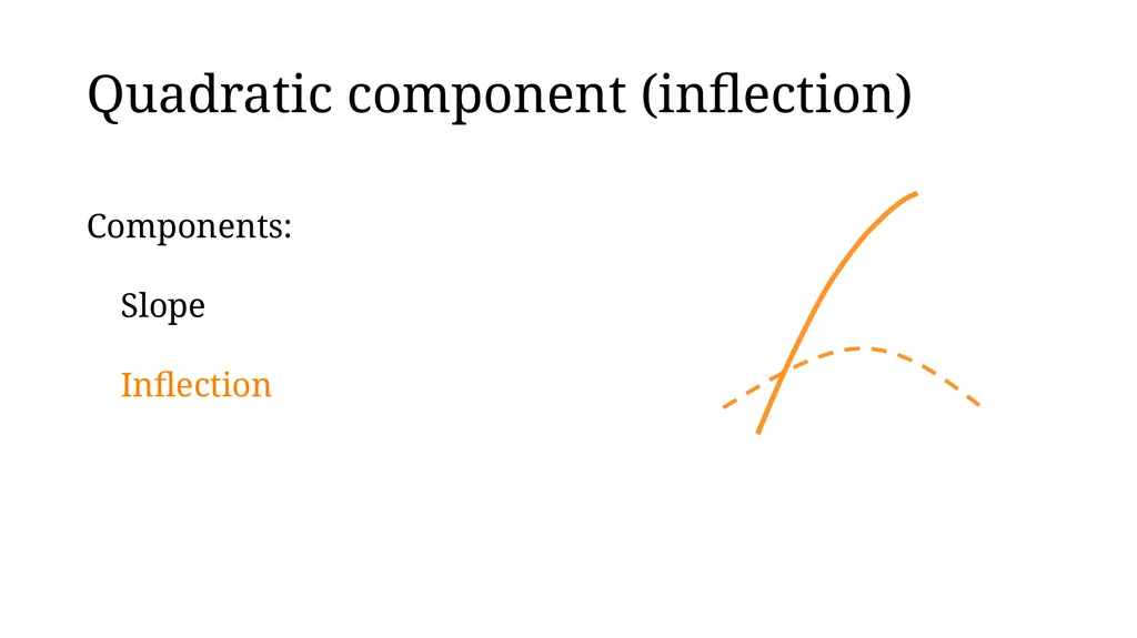
slide14. Quadratic component (inflection) Components:

Slope

Inflection<br>
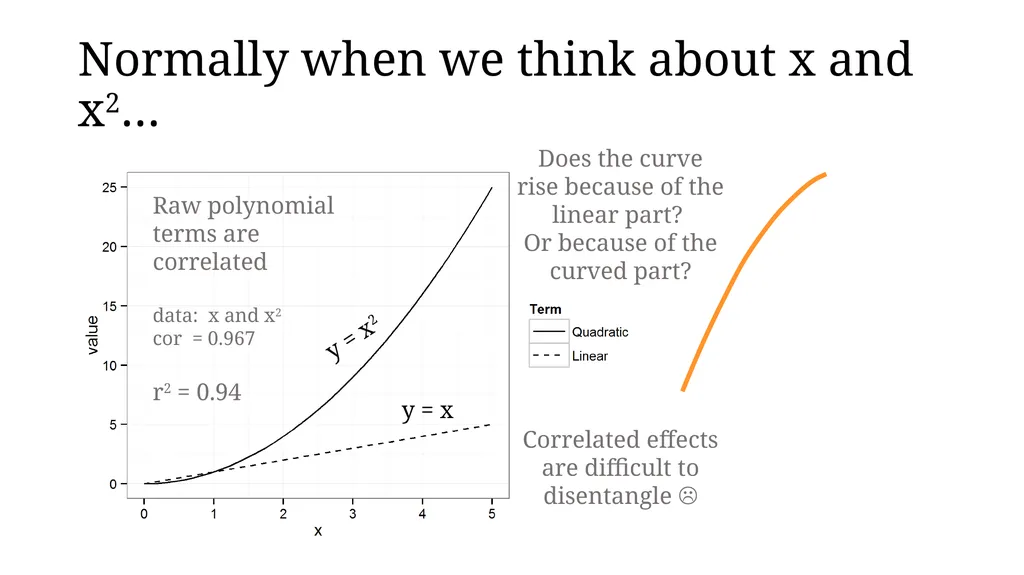
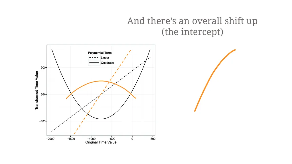
slide15. Normally when we think about x and x2… Raw polynomial terms are correlated

data: x and x2
cor = 0.967

r2 = 0.94 Does the curve rise because of the linear part? Or because of the curved part?

Correlated effects are difficult to disentangle <br>
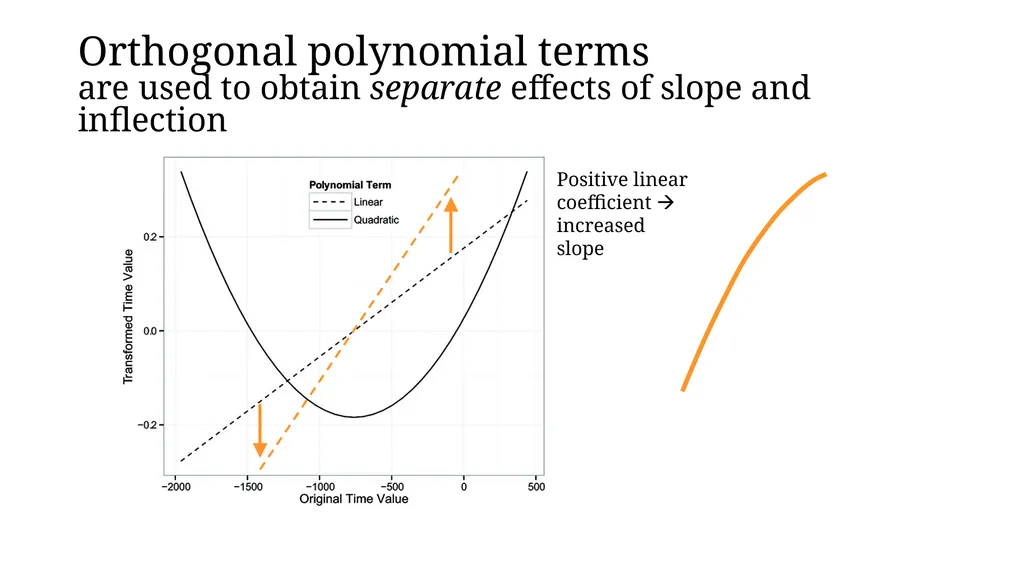
slide16. Orthogonal polynomial termsare used to obtain separate effects of slope and inflection Positive linear coefficient  increased slope<br>
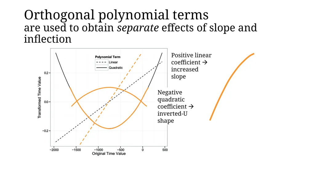
slide17. Orthogonal polynomial termsare used to obtain separate effects of slope and inflection e e Positive linear coefficient  increased slope Negative quadratic coefficient  inverted-U shape<br>
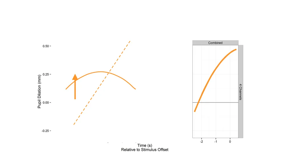
slide18. And there’s an overall shift up
(the intercept)<br>
slide19. Now that we have these components, let’s see how they contribute to the whole.<br>
slide20. e<br>
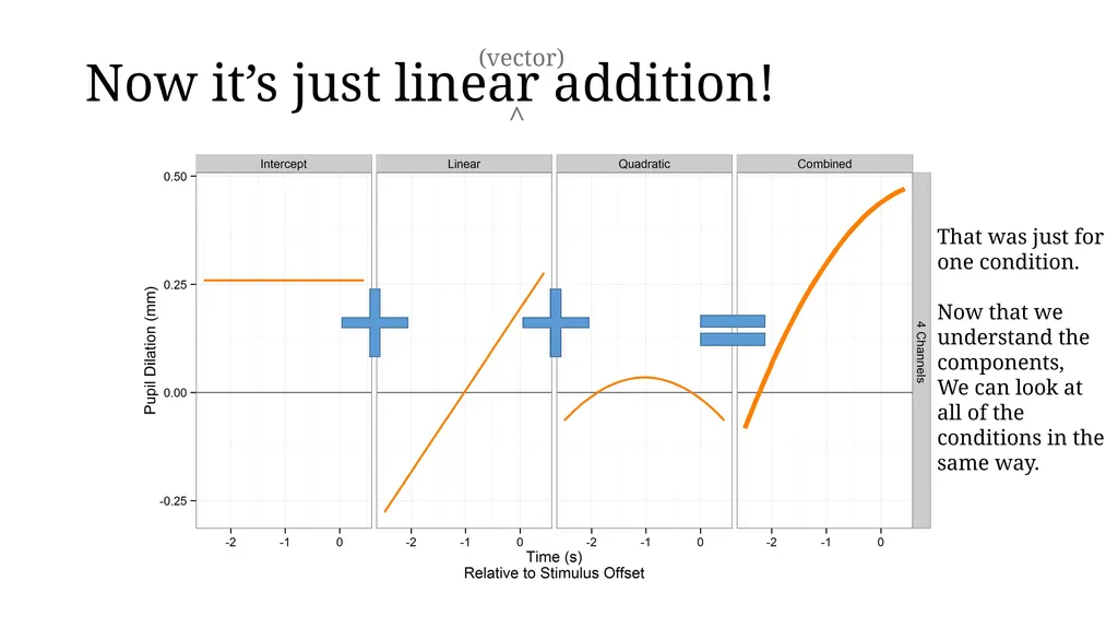
slide21. Now it’s just linear addition! That was just for one condition.

Now that we understand the components, We can look at all of the conditions in the same way. (vector)

^<br>
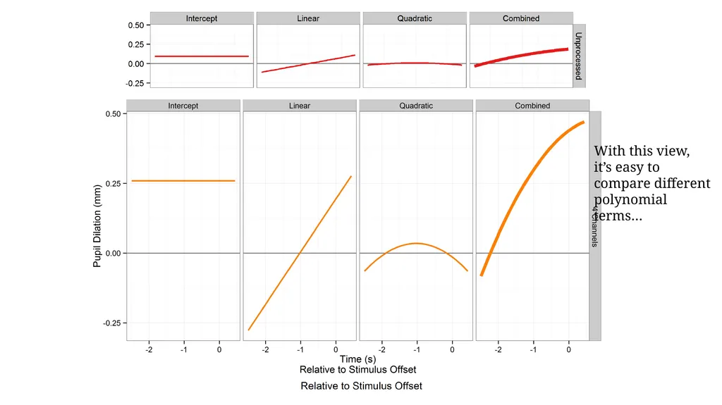
slide22. With this view, it’s easy to compare different polynomial terms…<br>
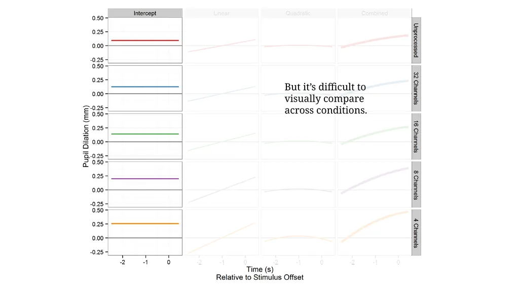
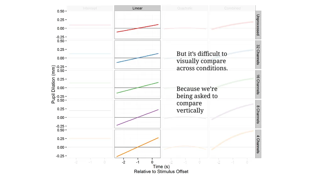
slide23. But it’s difficult to visually compare across conditions.<br>
slide24. But it’s difficult to visually compare across conditions. Because we’re being asked to compare vertically<br>
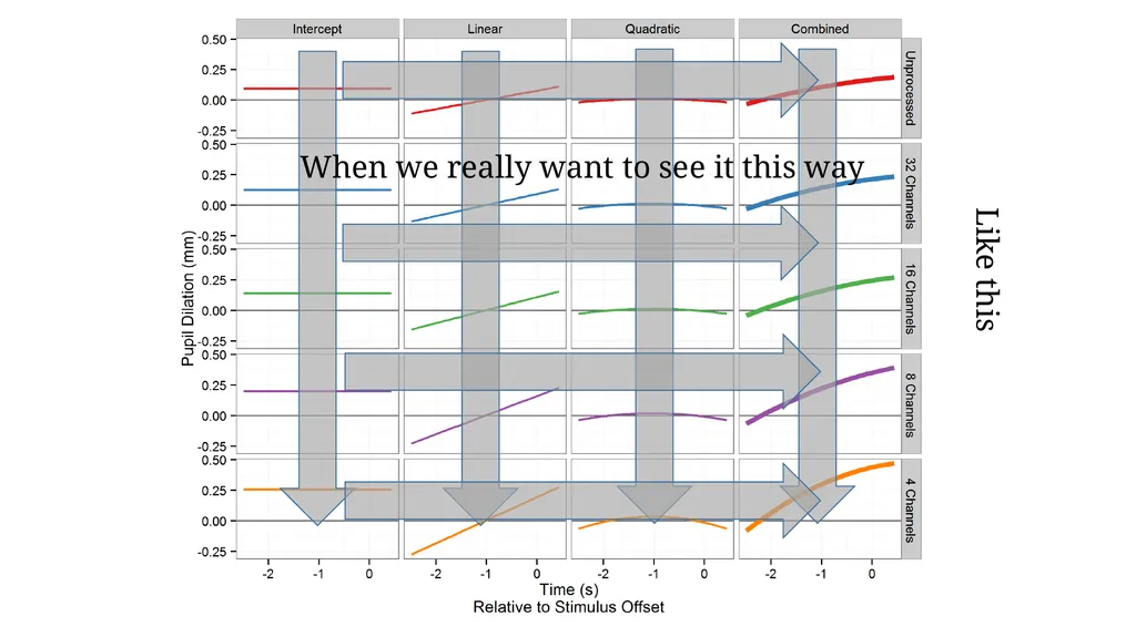
slide25. Like this When we really want to see it this way<br>
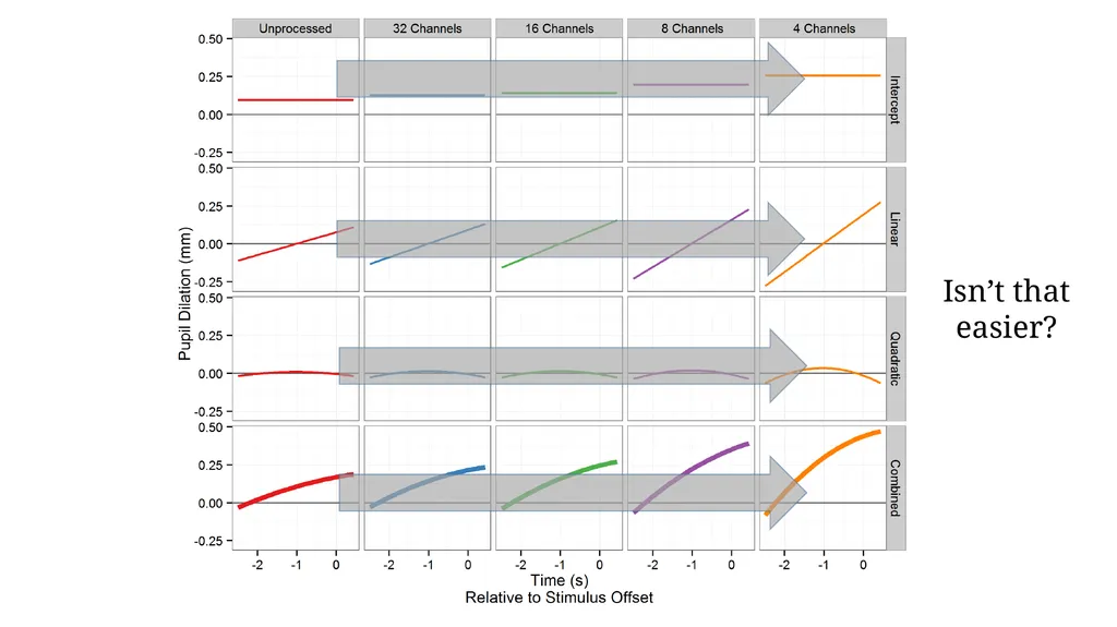
slide26. Isn’t that easier?<br>
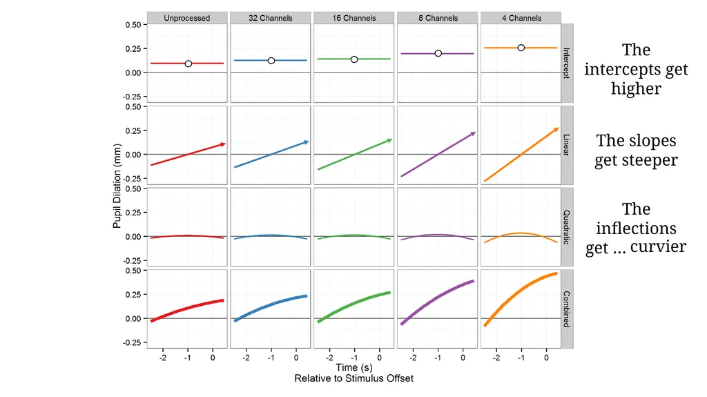
slide27. The intercepts get higher The slopesget steeper The inflectionsget … curvier curvier<br>
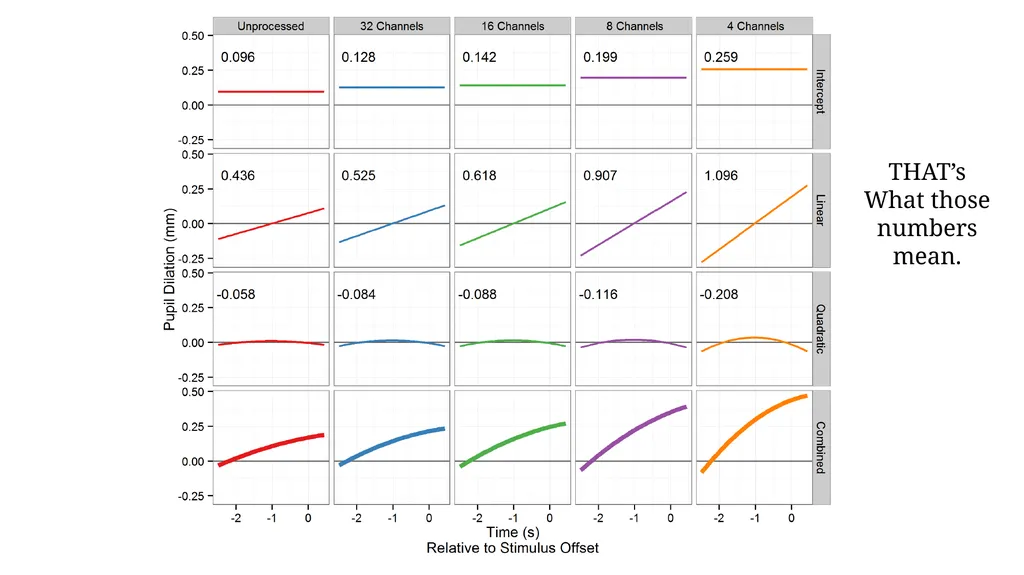
slide28. THAT’s
What those numbers mean.<br>
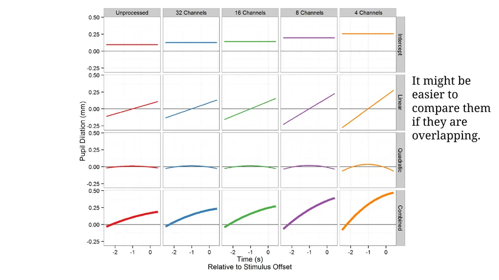
slide29. It might be easier to compare them if they are overlapping.<br>
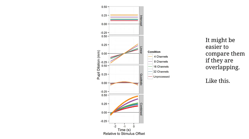
slide30. It might be easier to compare them if they are overlapping.

Like this.<br>
slide31. Or, if you’re horizontally inclined…<br>
slide32. Or, if you’re horizontally inclined… Notice how we can now compare slopes without being distractedby differences in overall height<br>
slide33. Now we’ve learned the connection between THIS and THIS<br>
slide34. The End.<br>