
Lecture 2- NumPy I 1 Dr. Sampath Jayarathna Old

Description: Lecture 2- NumPy I 1 Dr. Sampath Jayarathna Old Dominion University Credit for some of the slides in this lecture goes to Jianhua Ruan UTSA CS 620 DASC 600 Introduction to Data Science Analytics NumPy Stands for Numerical Python Is the
Related Topics
Download Presentation
"Lecture 2- NumPy I 1 Dr. Sampath Jayarathna Old" is the property of its rightful owner. Permission is granted to download and print the materials on this website for personal, non-commercial use only, and to display it on your personal computer provided you do not modify the materials and that you retain all copyright notices contained in the materials. By downloading content from our website, you accept the terms of this agreement.
Presentation Transcript
slide1. Lecture 2- NumPy I 1 Dr. Sampath Jayarathna
Old Dominion University Credit for some of the slides in this lecture goes to Jianhua Ruan UTSA CS 620 / DASC 600
Introduction to Data Science & Analytics<br>
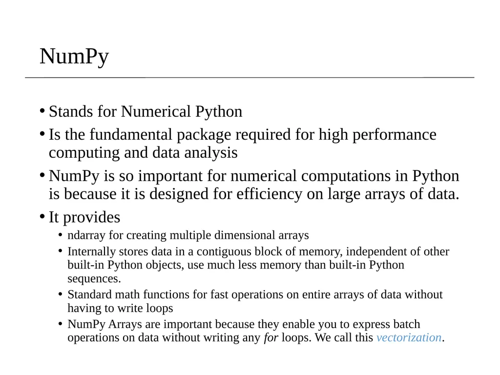
slide2. NumPy Stands for Numerical Python
Is the fundamental package required for high performance computing and data analysis
NumPy is so important for numerical computations in Python is because it is designed for efficiency on large arrays of data.
It provides
ndarray for creating multiple dimensional arrays
Internally stores data in a contiguous block of memory, independent of other built-in Python objects, use much less memory than built-in Python sequences.
Standard math functions for fast operations on entire arrays of data without having to write loops
NumPy Arrays are important because they enable you to express batch operations on data without writing any for loops. We call this vectorization.<br>
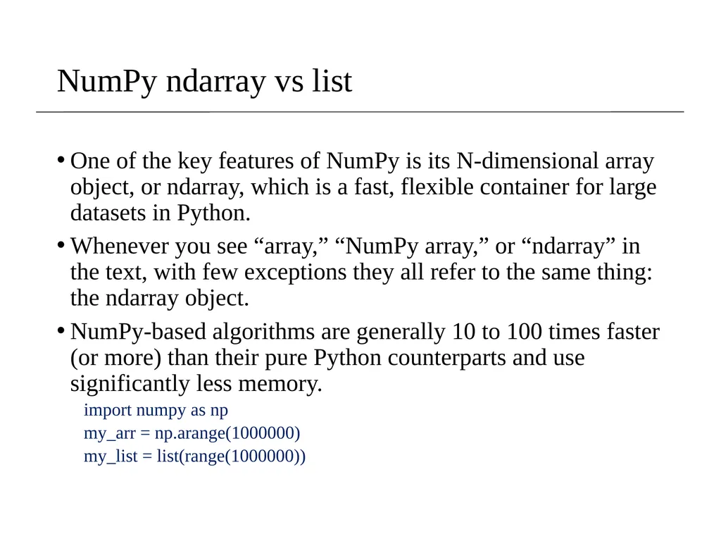
slide3. NumPy ndarray vs list One of the key features of NumPy is its N-dimensional array object, or ndarray, which is a fast, flexible container for large datasets in Python.
Whenever you see “array,” “NumPy array,” or “ndarray” in the text, with few exceptions they all refer to the same thing: the ndarray object.
NumPy-based algorithms are generally 10 to 100 times faster (or more) than their pure Python counterparts and use significantly less memory.
import numpy as np
my_arr = np.arange(1000000)
my_list = list(range(1000000))<br>
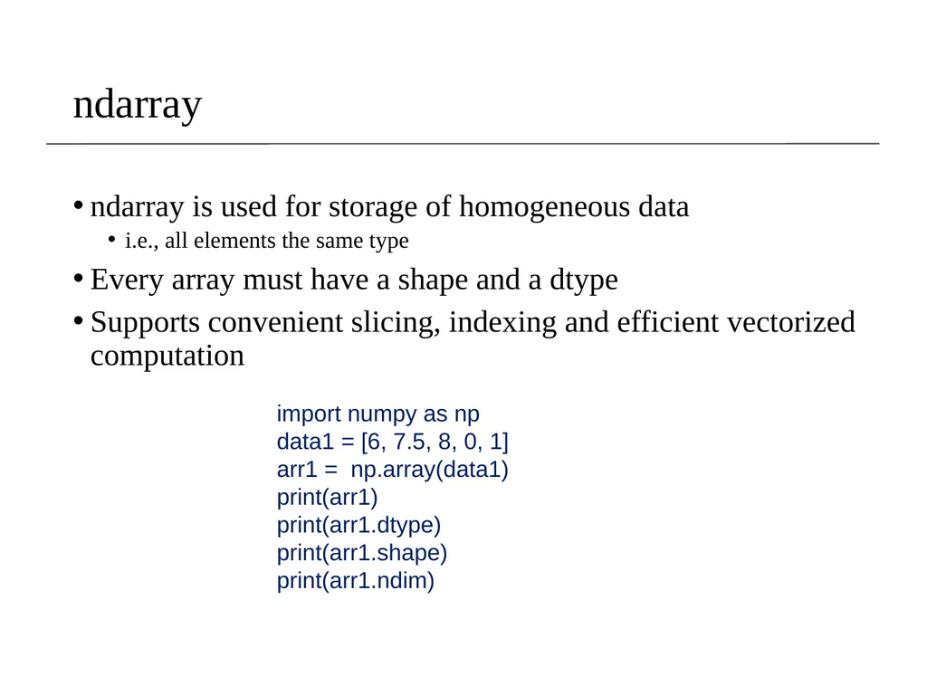
slide4. ndarray ndarray is used for storage of homogeneous data
i.e., all elements the same type
Every array must have a shape and a dtype
Supports convenient slicing, indexing and efficient vectorized computation import numpy as np
data1 = [6, 7.5, 8, 0, 1]
arr1 = np.array(data1)
print(arr1)
print(arr1.dtype)
print(arr1.shape)
print(arr1.ndim)<br>
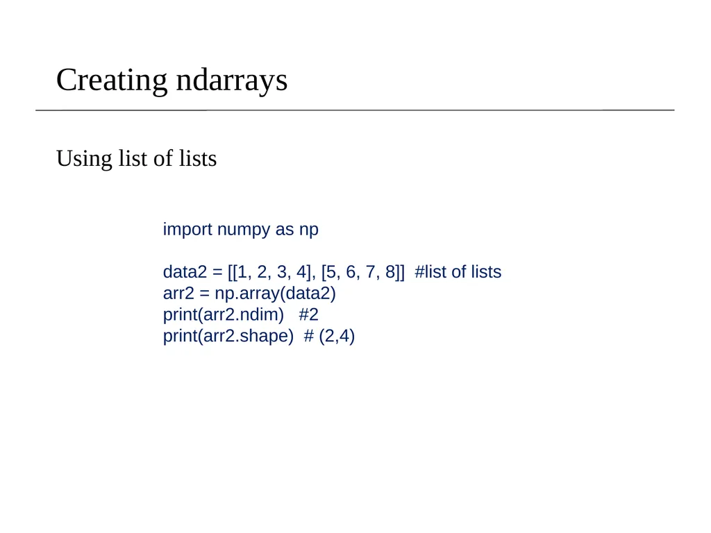
slide5. Creating ndarrays Using list of lists import numpy as np
data2 = [[1, 2, 3, 4], [5, 6, 7, 8]] #list of lists
arr2 = np.array(data2)
print(arr2.ndim) #2
print(arr2.shape) # (2,4)<br>
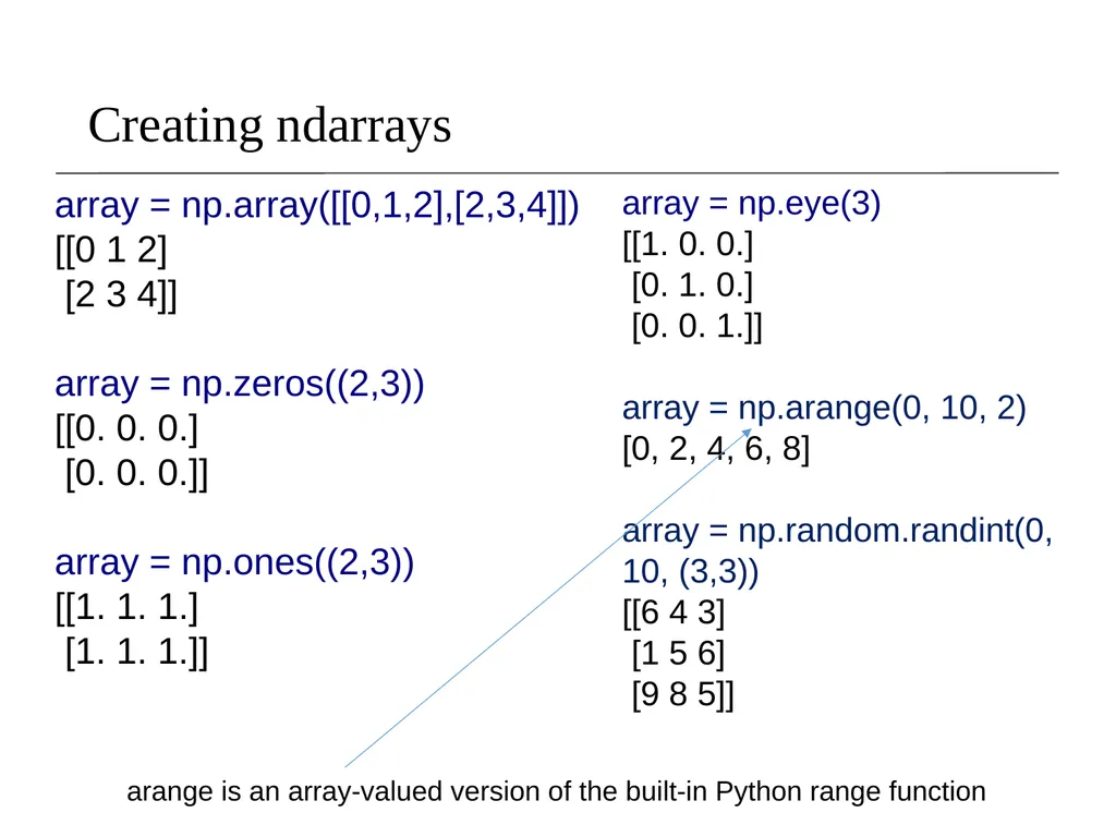
slide6. array = np.array([[0,1,2],[2,3,4]])
[[0 1 2]
[2 3 4]]
array = np.zeros((2,3))
[[0. 0. 0.]
[0. 0. 0.]]
array = np.ones((2,3))
[[1. 1. 1.]
[1. 1. 1.]] array = np.eye(3)
[[1. 0. 0.]
[0. 1. 0.]
[0. 0. 1.]]
array = np.arange(0, 10, 2)
[0, 2, 4, 6, 8]
array = np.random.randint(0, 10, (3,3))
[[6 4 3]
[1 5 6]
[9 8 5]] Creating ndarrays arange is an array-valued version of the built-in Python range function<br>
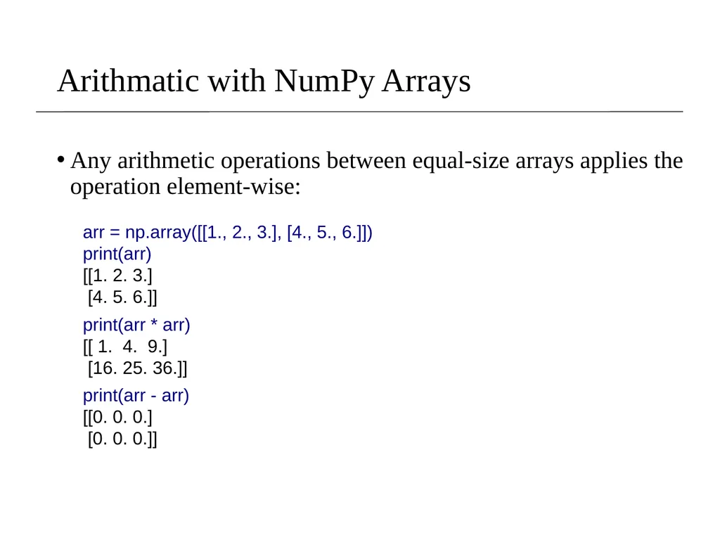
slide7. Arithmatic with NumPy Arrays Any arithmetic operations between equal-size arrays applies the operation element-wise: arr = np.array([[1., 2., 3.], [4., 5., 6.]])
print(arr)
[[1. 2. 3.]
[4. 5. 6.]]
print(arr * arr)
[[ 1. 4. 9.]
[16. 25. 36.]]
print(arr - arr)
[[0. 0. 0.]
[0. 0. 0.]]<br>
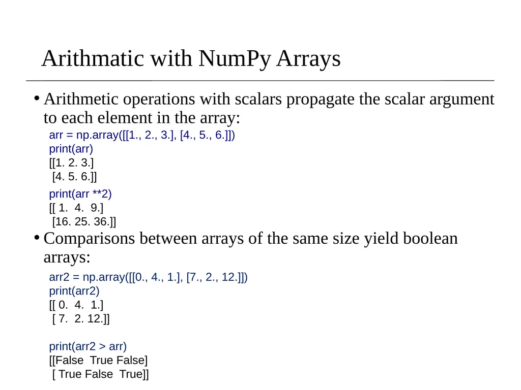
slide8. Arithmatic with NumPy Arrays Arithmetic operations with scalars propagate the scalar argument to each element in the array:
Comparisons between arrays of the same size yield boolean arrays: arr = np.array([[1., 2., 3.], [4., 5., 6.]])
print(arr)
[[1. 2. 3.]
[4. 5. 6.]]
print(arr **2)
[[ 1. 4. 9.]
[16. 25. 36.]]
arr2 = np.array([[0., 4., 1.], [7., 2., 12.]])
print(arr2)
[[ 0. 4. 1.]
[ 7. 2. 12.]]
print(arr2 > arr)
[[False True False]
[ True False True]]<br>
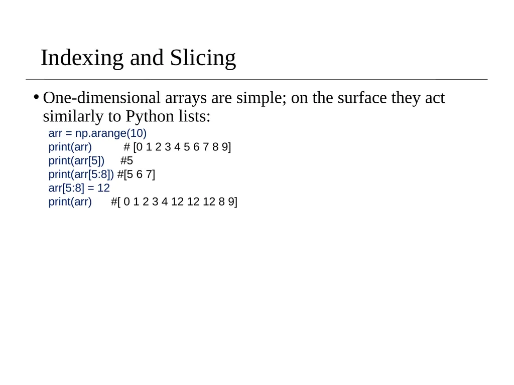
slide9. Indexing and Slicing One-dimensional arrays are simple; on the surface they act similarly to Python lists: arr = np.arange(10)
print(arr) # [0 1 2 3 4 5 6 7 8 9]
print(arr[5]) #5
print(arr[5:8]) #[5 6 7]
arr[5:8] = 12
print(arr) #[ 0 1 2 3 4 12 12 12 8 9]<br>
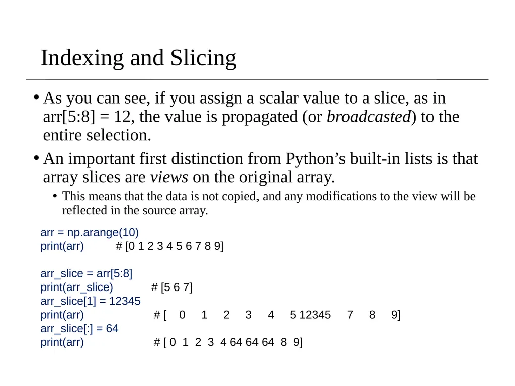
slide10. Indexing and Slicing As you can see, if you assign a scalar value to a slice, as in arr[5:8] = 12, the value is propagated (or broadcasted) to the entire selection.
An important first distinction from Python’s built-in lists is that array slices are views on the original array.
This means that the data is not copied, and any modifications to the view will be reflected in the source array. arr = np.arange(10)
print(arr) # [0 1 2 3 4 5 6 7 8 9]
arr_slice = arr[5:8]
print(arr_slice) # [5 6 7]
arr_slice[1] = 12345
print(arr) # [ 0 1 2 3 4 5 12345 7 8 9]
arr_slice[:] = 64
print(arr) # [ 0 1 2 3 4 64 64 64 8 9]<br>
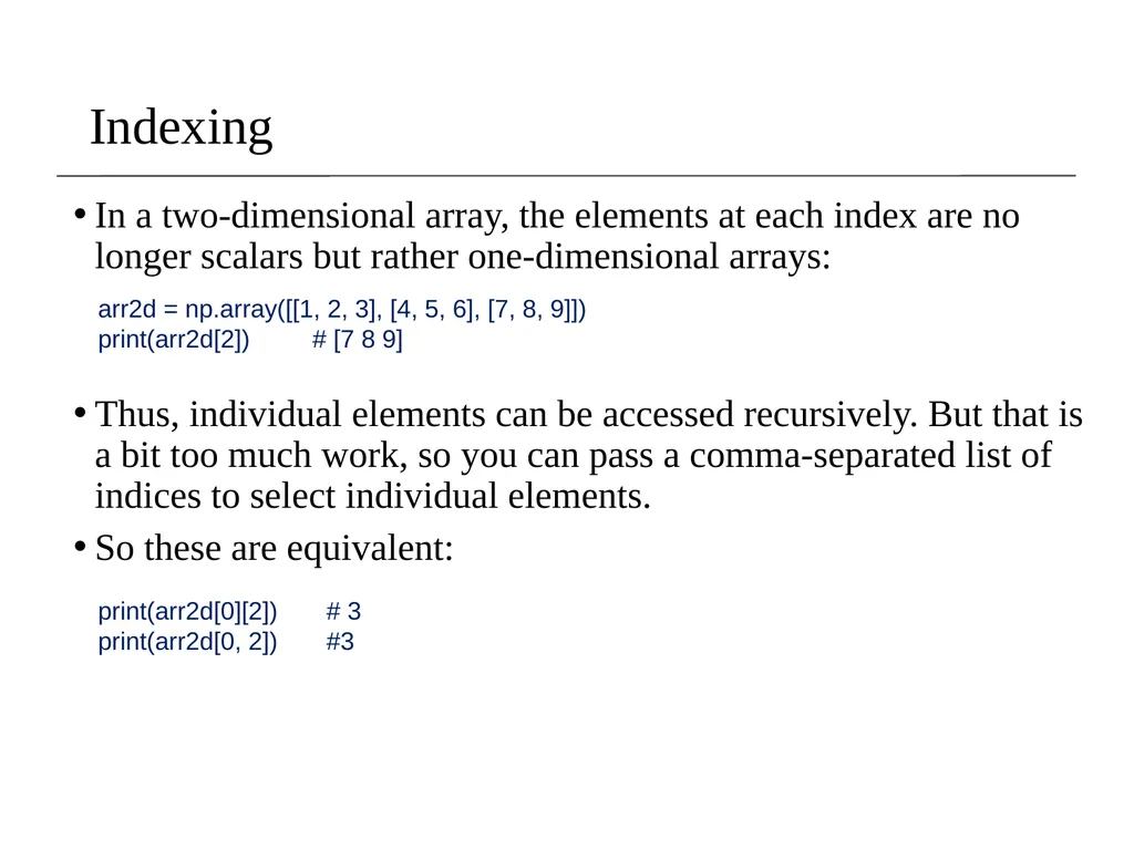
slide11. Indexing In a two-dimensional array, the elements at each index are no longer scalars but rather one-dimensional arrays:
Thus, individual elements can be accessed recursively. But that is a bit too much work, so you can pass a comma-separated list of indices to select individual elements.
So these are equivalent: arr2d = np.array([[1, 2, 3], [4, 5, 6], [7, 8, 9]])
print(arr2d[2]) # [7 8 9]
print(arr2d[0][2]) # 3
print(arr2d[0, 2]) #3<br>
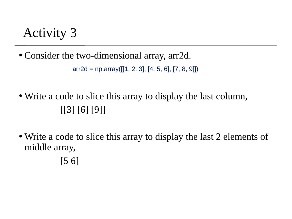
slide12. Activity 3 Consider the two-dimensional array, arr2d.
Write a code to slice this array to display the last column,
[[3] [6] [9]]
Write a code to slice this array to display the last 2 elements of middle array,
[5 6] arr2d = np.array([[1, 2, 3], [4, 5, 6], [7, 8, 9]])<br>
Old Dominion University Credit for some of the slides in this lecture goes to Jianhua Ruan UTSA CS 620 / DASC 600
Introduction to Data Science & Analytics<br>
slide2. NumPy Stands for Numerical Python
Is the fundamental package required for high performance computing and data analysis
NumPy is so important for numerical computations in Python is because it is designed for efficiency on large arrays of data.
It provides
ndarray for creating multiple dimensional arrays
Internally stores data in a contiguous block of memory, independent of other built-in Python objects, use much less memory than built-in Python sequences.
Standard math functions for fast operations on entire arrays of data without having to write loops
NumPy Arrays are important because they enable you to express batch operations on data without writing any for loops. We call this vectorization.<br>
slide3. NumPy ndarray vs list One of the key features of NumPy is its N-dimensional array object, or ndarray, which is a fast, flexible container for large datasets in Python.
Whenever you see “array,” “NumPy array,” or “ndarray” in the text, with few exceptions they all refer to the same thing: the ndarray object.
NumPy-based algorithms are generally 10 to 100 times faster (or more) than their pure Python counterparts and use significantly less memory.
import numpy as np
my_arr = np.arange(1000000)
my_list = list(range(1000000))<br>
slide4. ndarray ndarray is used for storage of homogeneous data
i.e., all elements the same type
Every array must have a shape and a dtype
Supports convenient slicing, indexing and efficient vectorized computation import numpy as np
data1 = [6, 7.5, 8, 0, 1]
arr1 = np.array(data1)
print(arr1)
print(arr1.dtype)
print(arr1.shape)
print(arr1.ndim)<br>
slide5. Creating ndarrays Using list of lists import numpy as np
data2 = [[1, 2, 3, 4], [5, 6, 7, 8]] #list of lists
arr2 = np.array(data2)
print(arr2.ndim) #2
print(arr2.shape) # (2,4)<br>
slide6. array = np.array([[0,1,2],[2,3,4]])
[[0 1 2]
[2 3 4]]
array = np.zeros((2,3))
[[0. 0. 0.]
[0. 0. 0.]]
array = np.ones((2,3))
[[1. 1. 1.]
[1. 1. 1.]] array = np.eye(3)
[[1. 0. 0.]
[0. 1. 0.]
[0. 0. 1.]]
array = np.arange(0, 10, 2)
[0, 2, 4, 6, 8]
array = np.random.randint(0, 10, (3,3))
[[6 4 3]
[1 5 6]
[9 8 5]] Creating ndarrays arange is an array-valued version of the built-in Python range function<br>
slide7. Arithmatic with NumPy Arrays Any arithmetic operations between equal-size arrays applies the operation element-wise: arr = np.array([[1., 2., 3.], [4., 5., 6.]])
print(arr)
[[1. 2. 3.]
[4. 5. 6.]]
print(arr * arr)
[[ 1. 4. 9.]
[16. 25. 36.]]
print(arr - arr)
[[0. 0. 0.]
[0. 0. 0.]]<br>
slide8. Arithmatic with NumPy Arrays Arithmetic operations with scalars propagate the scalar argument to each element in the array:
Comparisons between arrays of the same size yield boolean arrays: arr = np.array([[1., 2., 3.], [4., 5., 6.]])
print(arr)
[[1. 2. 3.]
[4. 5. 6.]]
print(arr **2)
[[ 1. 4. 9.]
[16. 25. 36.]]
arr2 = np.array([[0., 4., 1.], [7., 2., 12.]])
print(arr2)
[[ 0. 4. 1.]
[ 7. 2. 12.]]
print(arr2 > arr)
[[False True False]
[ True False True]]<br>
slide9. Indexing and Slicing One-dimensional arrays are simple; on the surface they act similarly to Python lists: arr = np.arange(10)
print(arr) # [0 1 2 3 4 5 6 7 8 9]
print(arr[5]) #5
print(arr[5:8]) #[5 6 7]
arr[5:8] = 12
print(arr) #[ 0 1 2 3 4 12 12 12 8 9]<br>
slide10. Indexing and Slicing As you can see, if you assign a scalar value to a slice, as in arr[5:8] = 12, the value is propagated (or broadcasted) to the entire selection.
An important first distinction from Python’s built-in lists is that array slices are views on the original array.
This means that the data is not copied, and any modifications to the view will be reflected in the source array. arr = np.arange(10)
print(arr) # [0 1 2 3 4 5 6 7 8 9]
arr_slice = arr[5:8]
print(arr_slice) # [5 6 7]
arr_slice[1] = 12345
print(arr) # [ 0 1 2 3 4 5 12345 7 8 9]
arr_slice[:] = 64
print(arr) # [ 0 1 2 3 4 64 64 64 8 9]<br>
slide11. Indexing In a two-dimensional array, the elements at each index are no longer scalars but rather one-dimensional arrays:
Thus, individual elements can be accessed recursively. But that is a bit too much work, so you can pass a comma-separated list of indices to select individual elements.
So these are equivalent: arr2d = np.array([[1, 2, 3], [4, 5, 6], [7, 8, 9]])
print(arr2d[2]) # [7 8 9]
print(arr2d[0][2]) # 3
print(arr2d[0, 2]) #3<br>
slide12. Activity 3 Consider the two-dimensional array, arr2d.
Write a code to slice this array to display the last column,
[[3] [6] [9]]
Write a code to slice this array to display the last 2 elements of middle array,
[5 6] arr2d = np.array([[1, 2, 3], [4, 5, 6], [7, 8, 9]])<br>