Numerical Methods for Describing Data From Graphical to Numerical 1. Traumatic knee dislocation often requires surgery to repair ruptured ligaments. One measure of recovery is range of motion (measured by the angle formed when, starting
"Numerical Methods for Describing Data From" is the property of its rightful owner. Permission is granted to
download and print the materials on this website for personal, non-commercial use only, and to display it
on your personal computer provided you do not modify the materials and that you retain all copyright
notices contained in the materials. By downloading content from our website, you accept the terms of this
agreement.
Presentation Transcript
01
Numerical Methods for Describing Data From Graphical to Numerical<br>
02
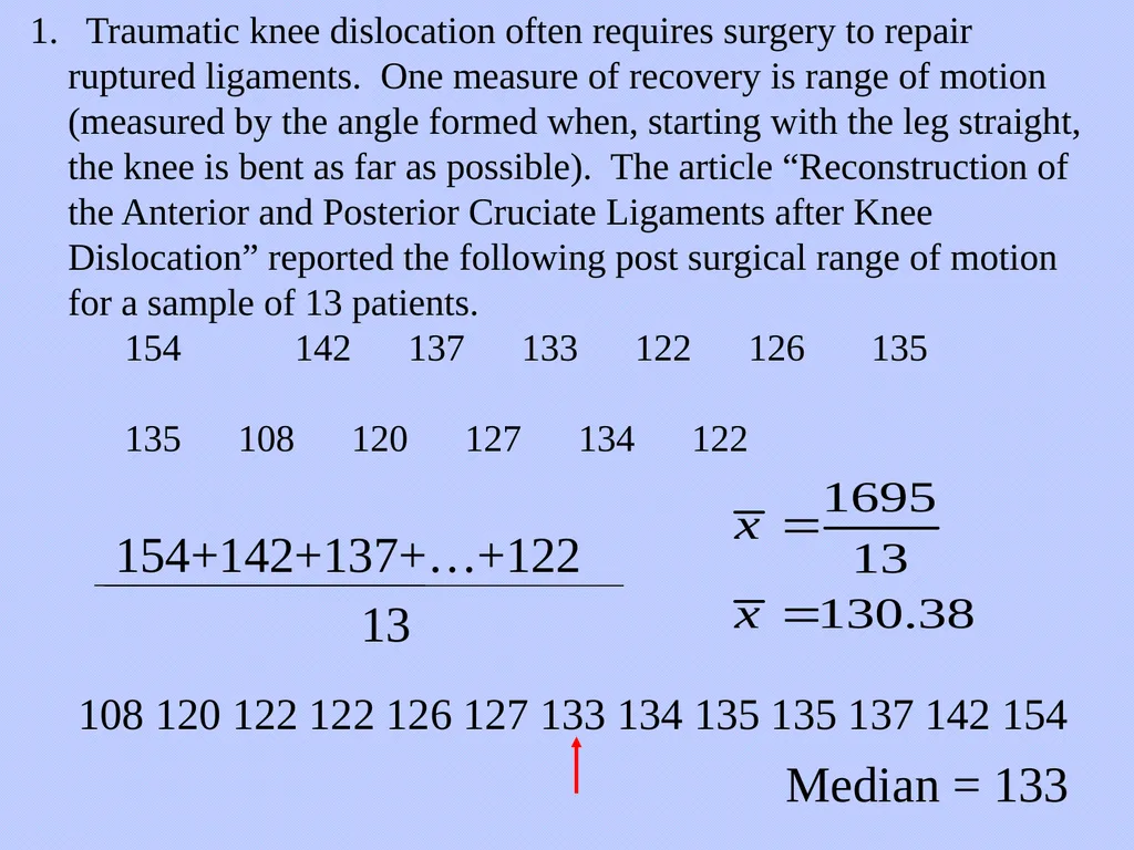
1. Traumatic knee dislocation often requires surgery to repair ruptured ligaments. One measure of recovery is range of motion (measured by the angle formed when, starting with the leg straight, the knee is bent as far as possible). The article “Reconstruction of the Anterior and Posterior Cruciate Ligaments after Knee Dislocation” reported the following post surgical range of motion for a sample of 13 patients.
142 137 133 122 126 135
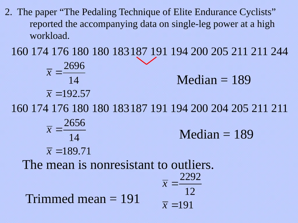
2. The paper “The Pedaling Technique of Elite Endurance Cyclists” reported the accompanying data on single-leg power at a high workload. 160 174 176 180 180 183 187 191 194 200 205 211 211 244 Median = 189 160 174 176 180 180 183 187 191 194 200 204 205 211 211 Median = 189 Trimmed mean = 191 The mean is nonresistant to outliers.<br>
04
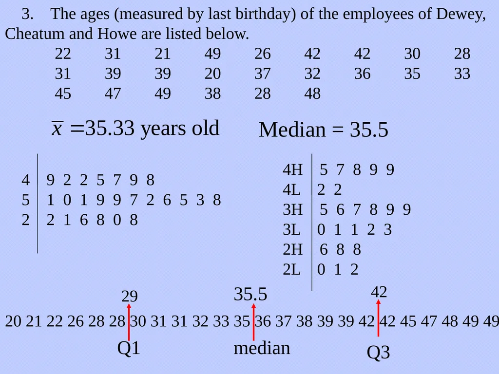
3. The ages (measured by last birthday) of the employees of Dewey, Cheatum and Howe are listed below.
22 31 21 49 26 42 42 30 28 31 39 39 20 37 32 36 35 33 45 47 49 38 28 48 Median = 35.5 20 21 22 26 28 28 30 31 31 32 33 35 36 37 38 39 39 42 42 45 47 48 49 49 Q1 Q3 35.5 median 29 42<br>
05
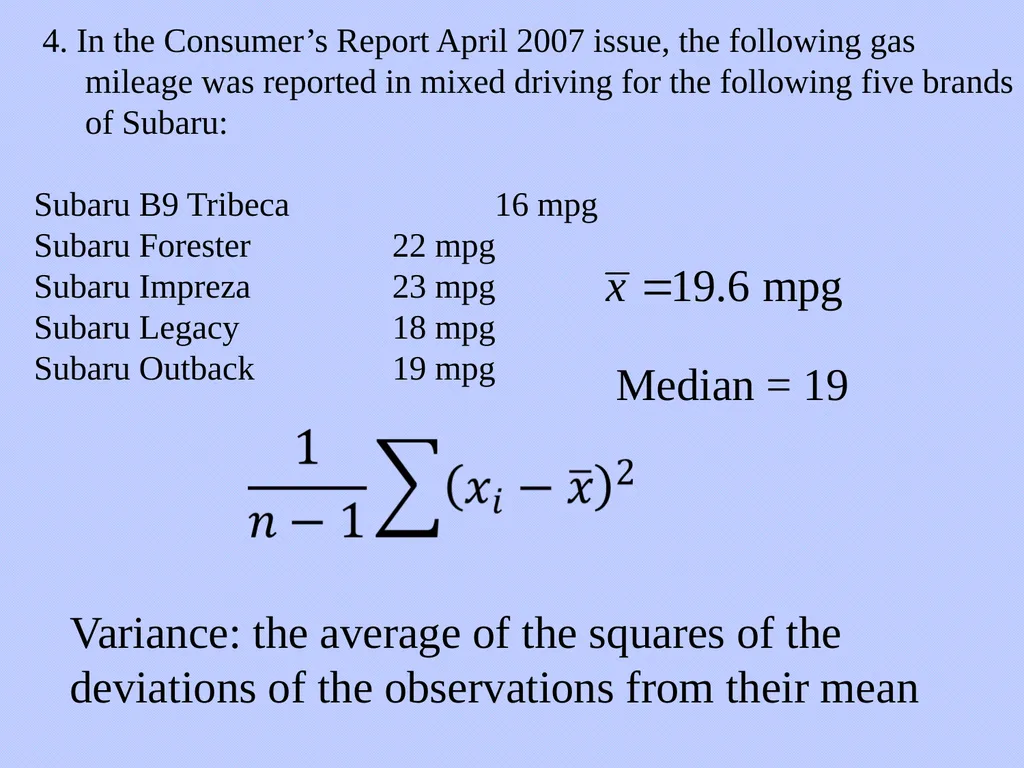
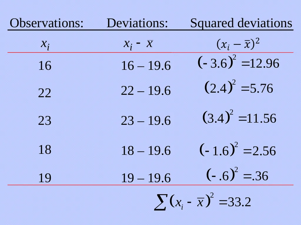
4. In the Consumer’s Report April 2007 issue, the following gas mileage was reported in mixed driving for the following five brands of Subaru:
Subaru B9 Tribeca 16 mpg
Subaru Forester 22 mpg
Subaru Impreza 23 mpg
Subaru Legacy 18 mpg
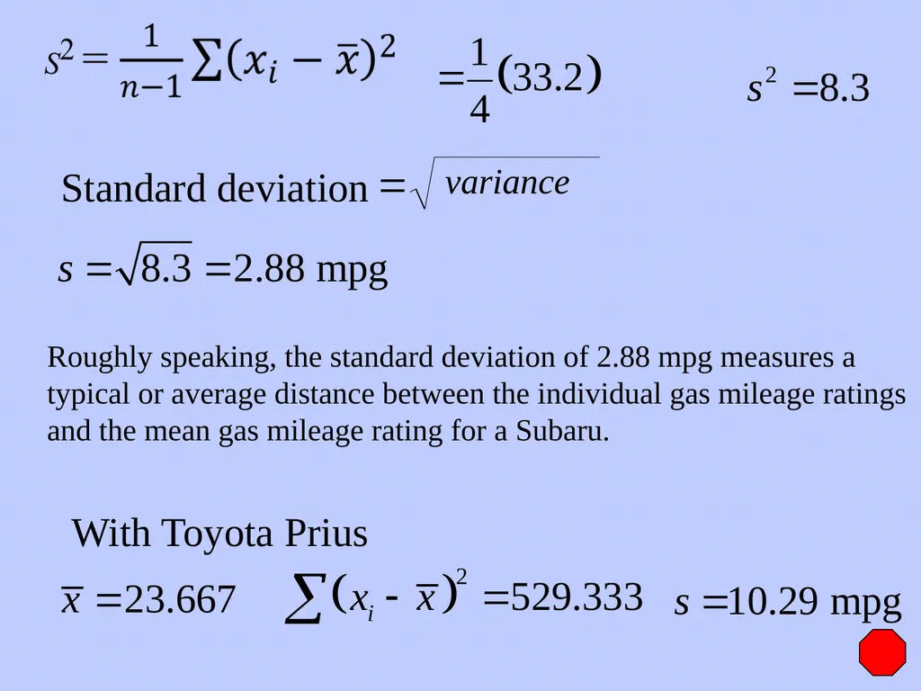
Subaru Outback 19 mpg Median = 19 Variance: the average of the squares of the deviations of the observations from their mean<br>
With Toyota Prius Roughly speaking, the standard deviation of 2.88 mpg measures a
typical or average distance between the individual gas mileage ratings
and the mean gas mileage rating for a Subaru.<br>
08
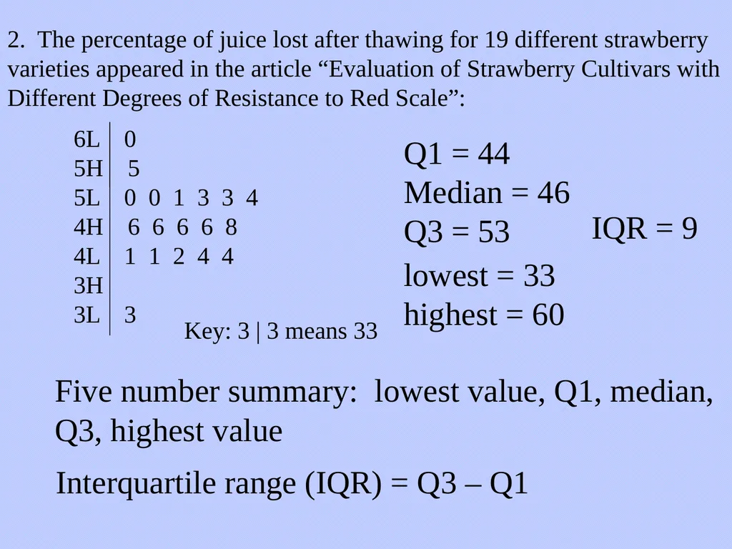
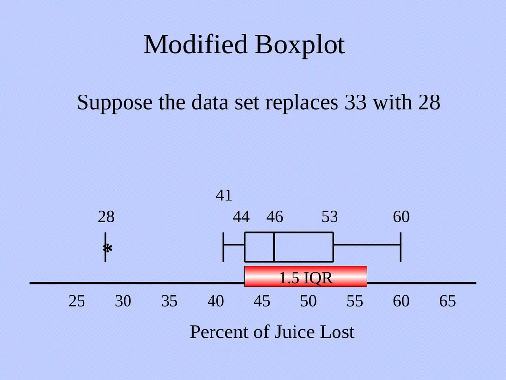
2. The percentage of juice lost after thawing for 19 different strawberry varieties appeared in the article “Evaluation of Strawberry Cultivars with Different Degrees of Resistance to Red Scale”: Q1 = 44
Median = 46
Q3 = 53 Five number summary: lowest value, Q1, median, Q3, highest value lowest = 33
highest = 60 Interquartile range (IQR) = Q3 – Q1 IQR = 9<br>
09
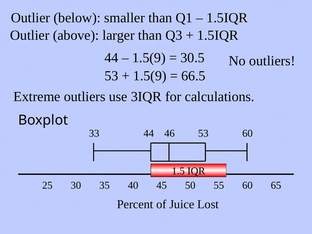
Outlier (below): smaller than Q1 – 1.5IQR 44 – 1.5(9) = 30.5 53 + 1.5(9) = 66.5 Extreme outliers use 3IQR for calculations. 25 30 35 40 45 50 55 60 65 Percent of Juice Lost No outliers! Boxplot IQR 1.5 IQR Outlier (above): larger than Q3 + 1.5IQR<br>
10
Modified Boxplot 25 30 35 40 45 50 55 60 65 28 Percent of Juice Lost 1.5 IQR Suppose the data set replaces 33 with 28 *<br>
11
Recap of Numerical Descriptors Measures of center: mean, median
Measures of variability: spread, range, IQR, variance, standard deviation
Mean, range, spread, variance and standard deviation are nonresistant to outliers.
How does shape affect the measures of center and variability?<br>
12
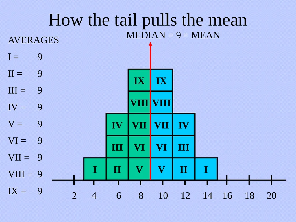
How the tail pulls the mean I I II V III VI VIII VII II VIII VII VI V III 2 4 6 8 10 12 14 16 18 20 MEDIAN = 9 AVERAGES
I = 9
II = 9
III = 9
IV = 9
V = 9
VI = 9
VII = 9
VIII = 9
IX = 9 IX IV IV IX = MEAN<br>
13
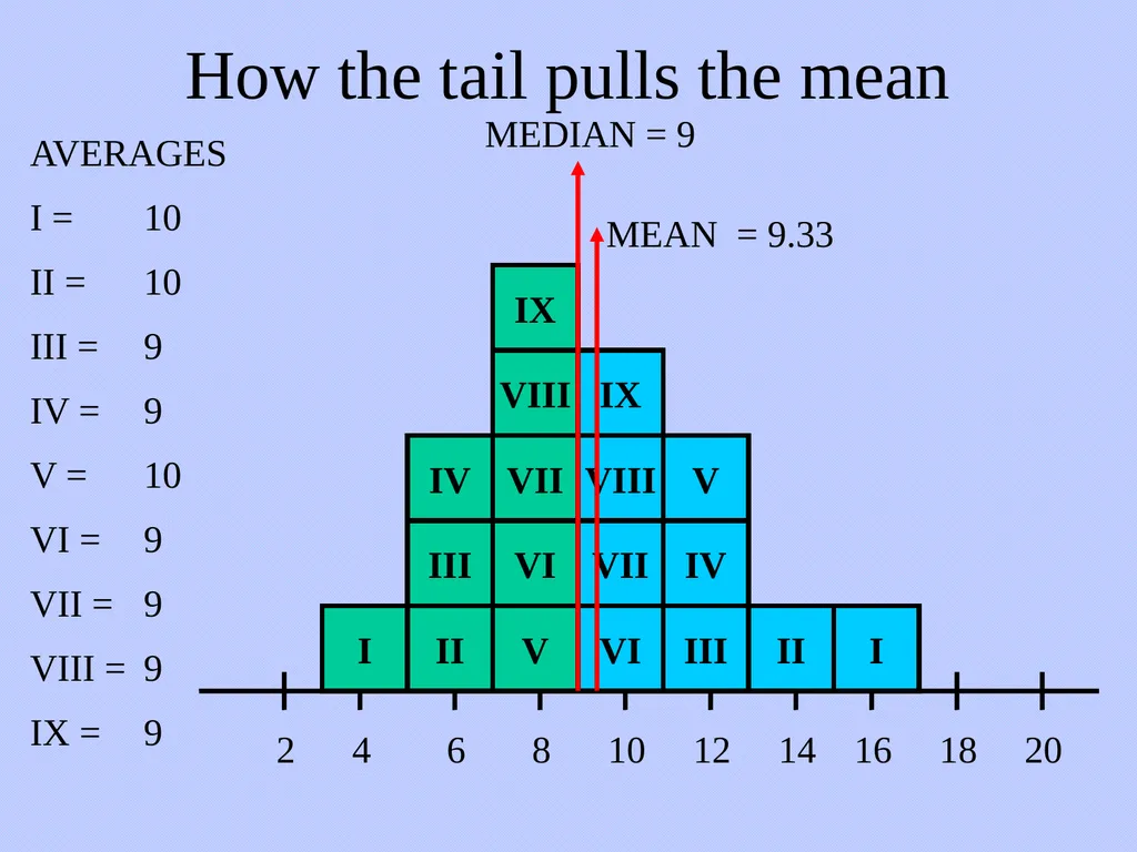
How the tail pulls the mean I I II V III VI VIII VII II VIII VII VI V III 2 4 6 8 10 12 14 16 18 20 MEDIAN = 9 AVERAGES
I = 10
II = 10
III = 9
IV = 9
V = 10
VI = 9
VII = 9
VIII = 9
IX = 9 IX IV IV IX<br>
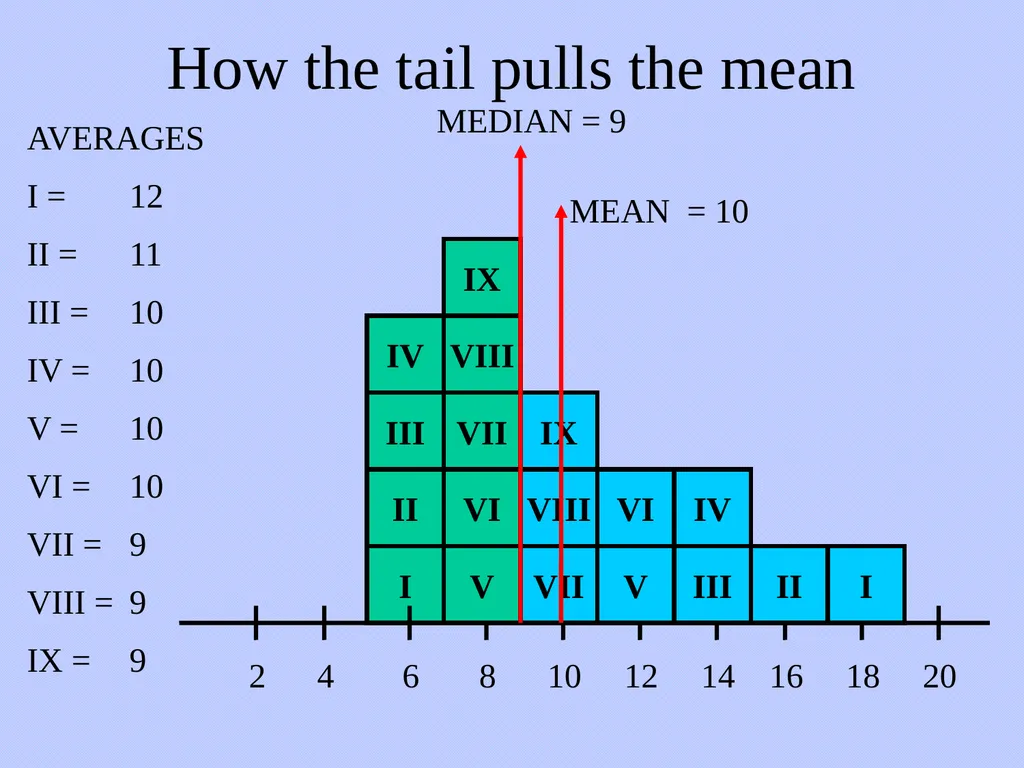
14
How the tail pulls the mean I I II V III VI VIII VII II VIII VII VI V III 2 4 6 8 10 12 14 16 18 20 MEDIAN = 9 AVERAGES
I = 12
II = 11
III = 10
IV = 10
V = 10
VI = 10
VII = 9
VIII = 9
IX = 9 IX IV IV IX<br>
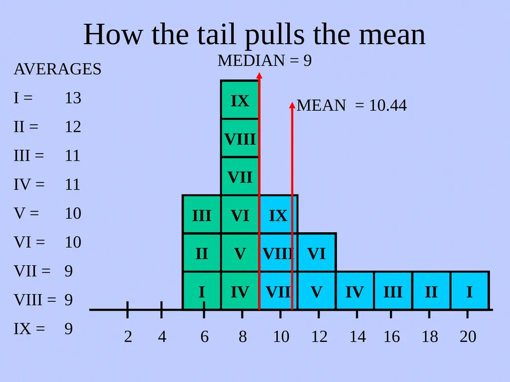
15
How the tail pulls the mean I I II V III VI VIII VII II VIII VII VI V III 2 4 6 8 10 12 14 16 18 20 MEDIAN = 9 AVERAGES
I = 13
II = 12
III = 11
IV = 11
V = 10
VI = 10
VII = 9
VIII = 9
IX = 9 IX IV IV IX<br>