Sample design and weights Lecture 2 Aims To

slide1. Sample design and weights Lecture 2<br>
slide2. Aims To understand the similarities and differences in the design of the key international surveys

To understand the response thresholds a country must meet for inclusion in the international reports.

To understand the design, purpose and appropriate use of the international assessment survey weights.

Introduce students to the use of ‘replication weights’ as a method for appropriately handling complex survey designs.

Gain experience of the application of such weights using the TALIS 2013 dataset.<br>
slide3. How are the large scale international studies designed?<br>
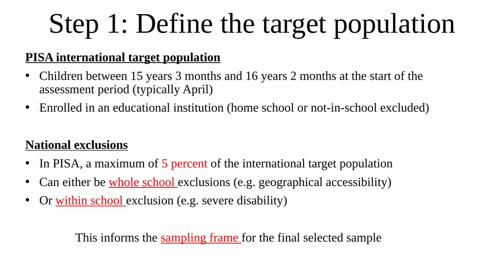
slide4. Step 1: Define the target population PISA international target population
Children between 15 years 3 months and 16 years 2 months at the start of the assessment period (typically April)
Enrolled in an educational institution (home school or not-in-school excluded)

National exclusions
In PISA, a maximum of 5 percent of the international target population
Can either be whole school exclusions (e.g. geographical accessibility)
Or within school exclusion (e.g. severe disability)

This informs the sampling frame for the final selected sample<br>
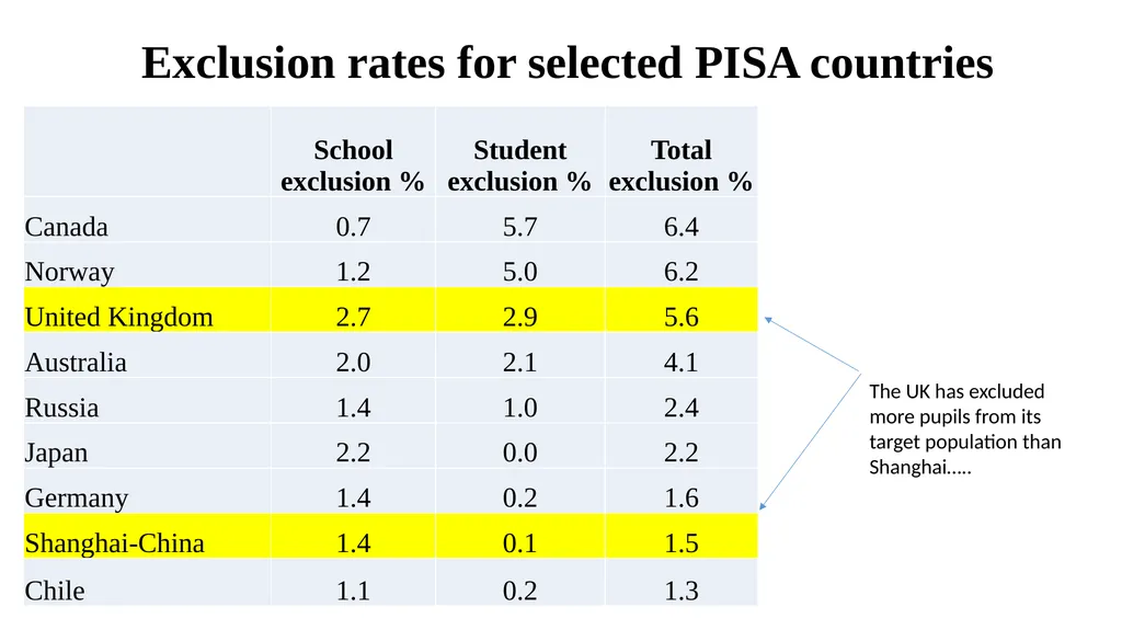
slide5. Exclusion rates for selected PISA countries The UK has excluded more pupils from its target population than Shanghai…..<br>
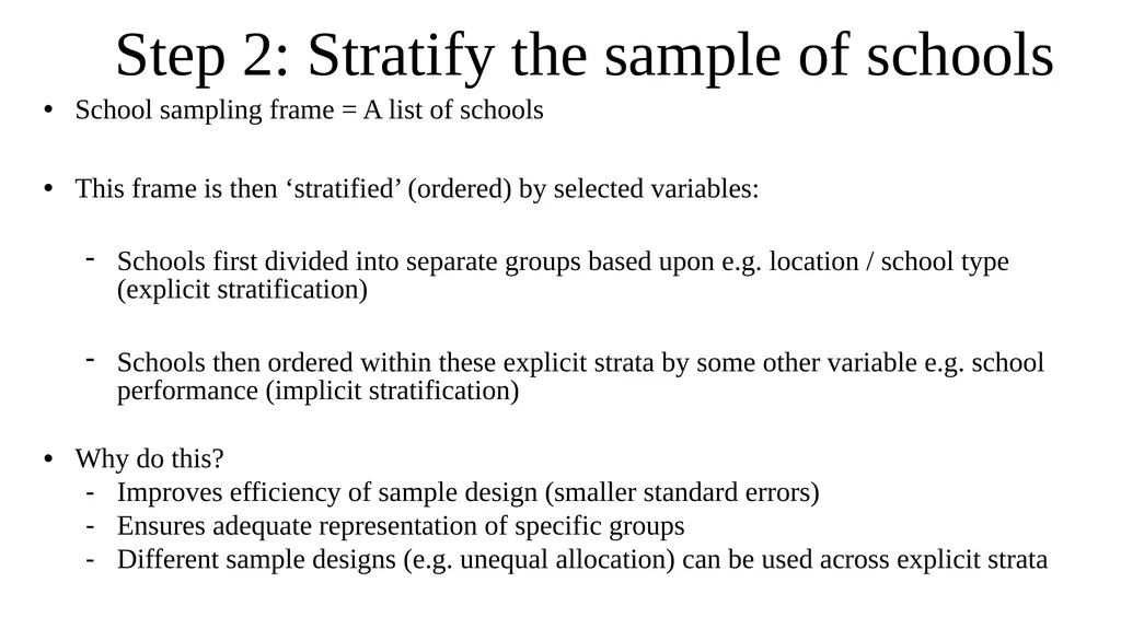
slide6. Step 2: Stratify the sample of schools School sampling frame = A list of schools

This frame is then ‘stratified’ (ordered) by selected variables:

Schools first divided into separate groups based upon e.g. location / school type (explicit stratification)

Schools then ordered within these explicit strata by some other variable e.g. school performance (implicit stratification)

Why do this?
Improves efficiency of sample design (smaller standard errors)
Ensures adequate representation of specific groups
Different sample designs (e.g. unequal allocation) can be used across explicit strata<br>
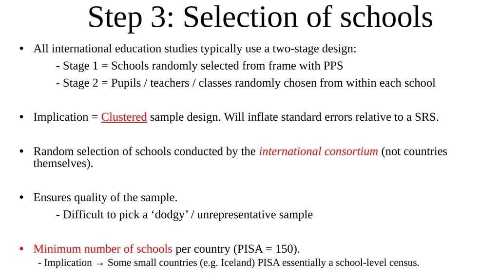
slide7. Step 3: Selection of schools All international education studies typically use a two-stage design:
- Stage 1 = Schools randomly selected from frame with PPS
- Stage 2 = Pupils / teachers / classes randomly chosen from within each school

Implication = Clustered sample design. Will inflate standard errors relative to a SRS.

Random selection of schools conducted by the international consortium (not countries themselves).

Ensures quality of the sample.
- Difficult to pick a ‘dodgy’ / unrepresentative sample

Minimum number of schools per country (PISA = 150).
- Implication → Some small countries (e.g. Iceland) PISA essentially a school-level census.<br>
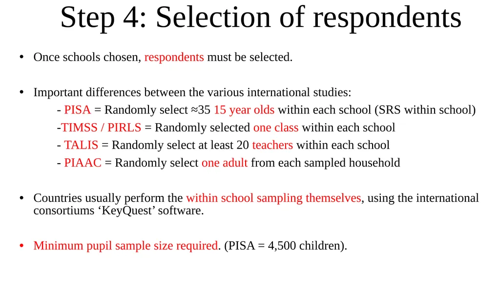
slide8. Step 4: Selection of respondents Once schools chosen, respondents must be selected.

Important differences between the various international studies:
- PISA = Randomly select ≈35 15 year olds within each school (SRS within school)
-TIMSS / PIRLS = Randomly selected one class within each school
- TALIS = Randomly select at least 20 teachers within each school
- PIAAC = Randomly select one adult from each sampled household

Countries usually perform the within school sampling themselves, using the international consortiums ‘KeyQuest’ software.

Minimum pupil sample size required. (PISA = 4,500 children).<br>
slide9. Non-response<br>
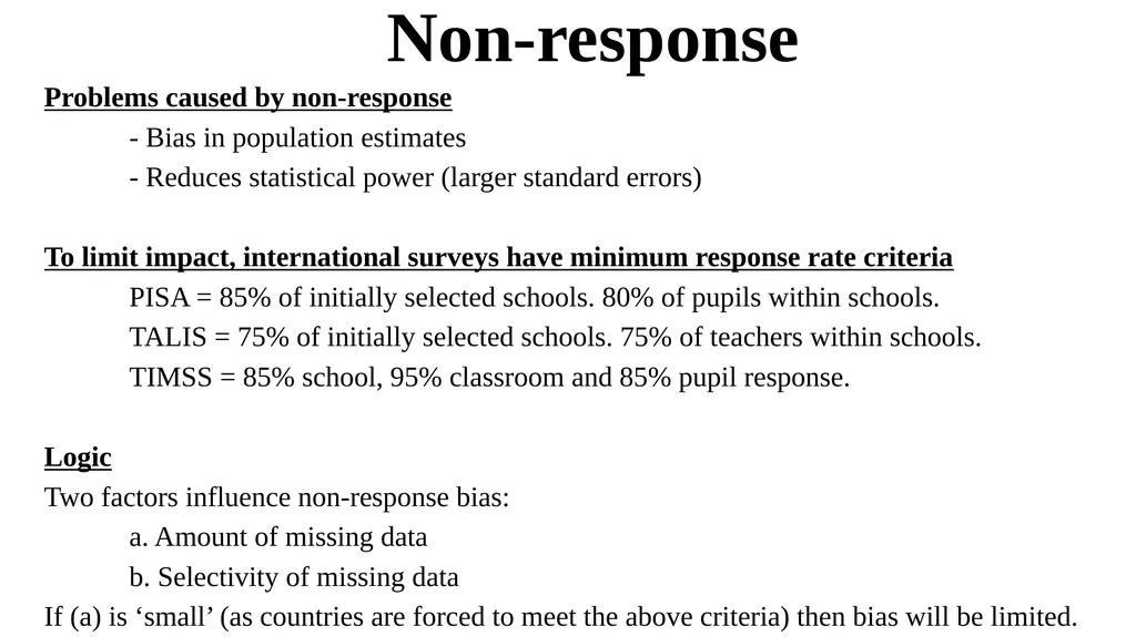
slide10. Non-response Problems caused by non-response
- Bias in population estimates
- Reduces statistical power (larger standard errors)

To limit impact, international surveys have minimum response rate criteria
PISA = 85% of initially selected schools. 80% of pupils within schools.
TALIS = 75% of initially selected schools. 75% of teachers within schools.
TIMSS = 85% school, 95% classroom and 85% pupil response.

Logic
Two factors influence non-response bias:
a. Amount of missing data
b. Selectivity of missing data
If (a) is ‘small’ (as countries are forced to meet the above criteria) then bias will be limited.<br>
slide11. ….but these ‘ideal’ criteria sometimes not met Source: TALIS 2013

School response rate required = 75%.

8 out of 34 countries did not meet this criteria<br>
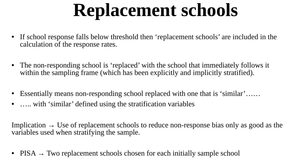
slide12. Replacement schools If school response falls below threshold then ‘replacement schools’ are included in the calculation of the response rates.

The non-responding school is ‘replaced’ with the school that immediately follows it within the sampling frame (which has been explicitly and implicitly stratified).

Essentially means non-responding school replaced with one that is ‘similar’……
….. with ‘similar’ defined using the stratification variables

Implication → Use of replacement schools to reduce non-response bias only as good as the variables used when stratifying the sample.

PISA → Two replacement schools chosen for each initially sample school<br>
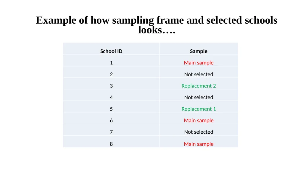
slide13. Example of how sampling frame and selected schools looks….<br>
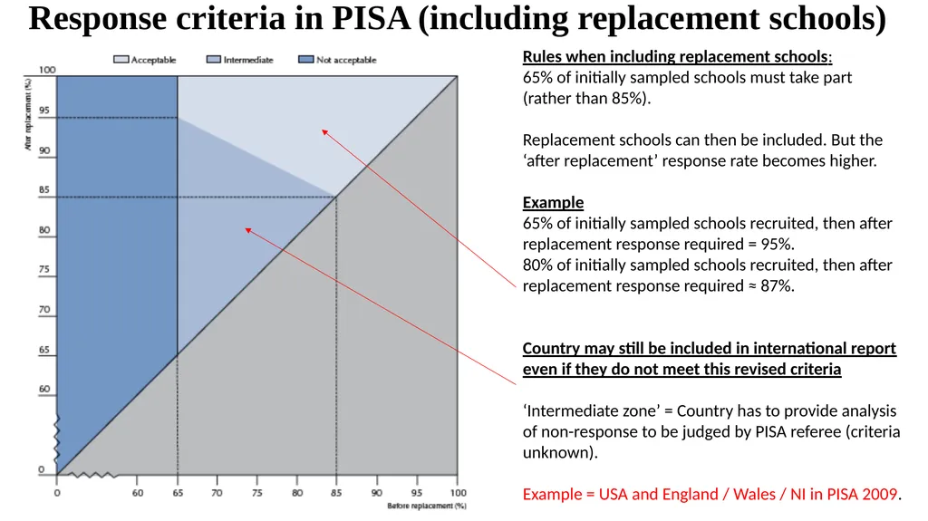
slide14. Response criteria in PISA (including replacement schools) Rules when including replacement schools:
65% of initially sampled schools must take part (rather than 85%).

Replacement schools can then be included. But the ‘after replacement’ response rate becomes higher.

Example
65% of initially sampled schools recruited, then after replacement response required = 95%.
80% of initially sampled schools recruited, then after replacement response required ≈ 87%.

Country may still be included in international report even if they do not meet this revised criteria

‘Intermediate zone’ = Country has to provide analysis of non-response to be judged by PISA referee (criteria unknown).

Example = USA and England / Wales / NI in PISA 2009.<br>
slide15. What do countries in the ‘intermediate’ zone provide? Example: US in 2009
Compared participating and non-participating schools in observable characteristics
Only those available on the sampling frame:
- School type; region; school size; ethnic composition; Free School Meals (FSM)

‘Bias’ based upon chi-square / t-test of difference between participants / non-participants
Found difference based upon FSM – but still included in the international report

Limitations of the bias analysis provided
Considers bias at school level only (not pupil level)
Small school level sample size (not enough power to detect important differences)
Very few characteristics considered<br>
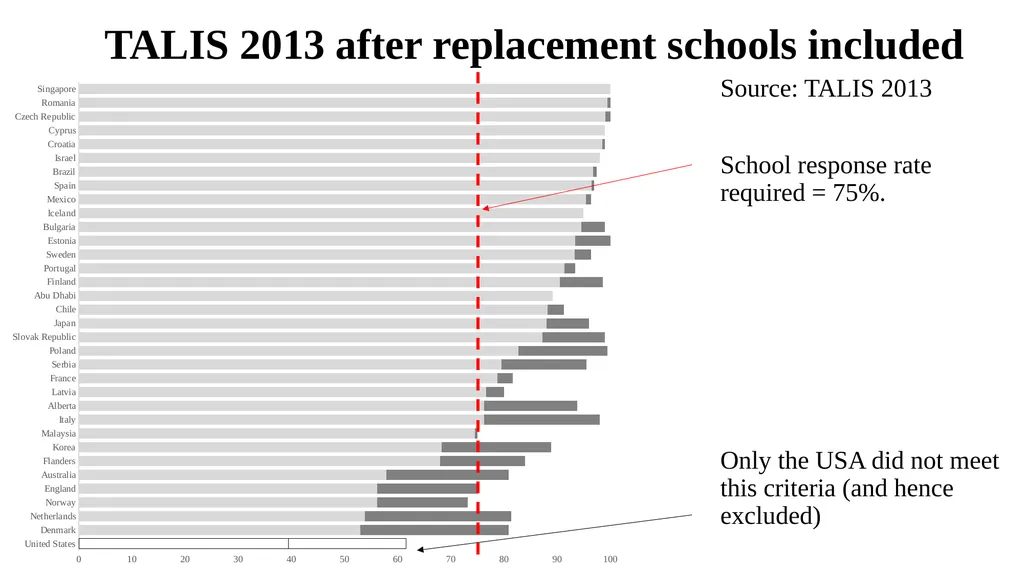
slide16. TALIS 2013 after replacement schools included Source: TALIS 2013

School response rate required = 75%.

Only the USA did not meet this criteria (and hence excluded)<br>
slide17. Implications of missing response target Kicked out of the international report (PISA/TALIS)
England/Wales/NI in PISA 2003
Netherlands TALIS 2008
United States TALIS 2013

Figures reported at bottom of table instead(TIMSS/PIRLS)
England in TIMSS 8th grade 2003

Exclusion from PISA 2003 national report described by Simon Briscoe, Economics Editor at The Financial Times, as among the ‘Top 20’ recent threats to public confidence in official statistics in the UK.

Being excluded still causing problems in UK politicians almost a decade later……<br>
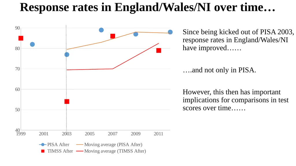
slide18. Response rates in England/Wales/NI over time… Since being kicked out of PISA 2003, response rates in England/Wales/NI have improved……

….and not only in PISA.

However, this then has important implications for comparisons in test scores over time……<br>
slide19. Respondent weights<br>
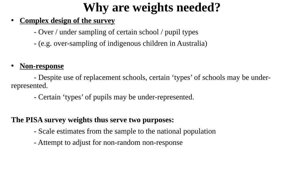
slide20. Why are weights needed? Complex design of the survey
- Over / under sampling of certain school / pupil types
- (e.g. over-sampling of indigenous children in Australia)

Non-response
- Despite use of replacement schools, certain ‘types’ of schools may be under- represented.
- Certain ‘types’ of pupils may be under-represented.

The PISA survey weights thus serve two purposes:
- Scale estimates from the sample to the national population
- Attempt to adjust for non-random non-response<br>
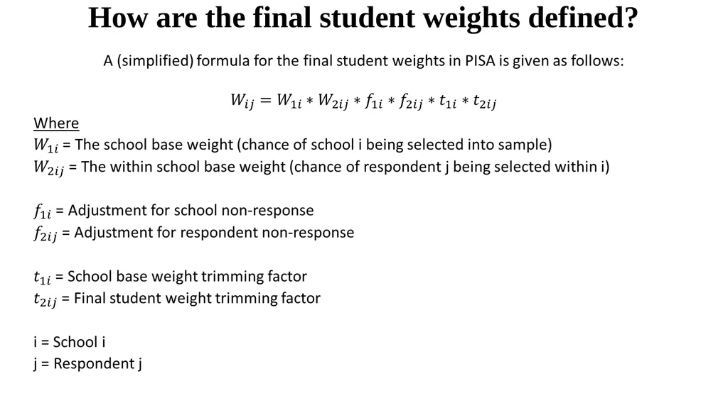
slide21. How are the final student weights defined?<br>
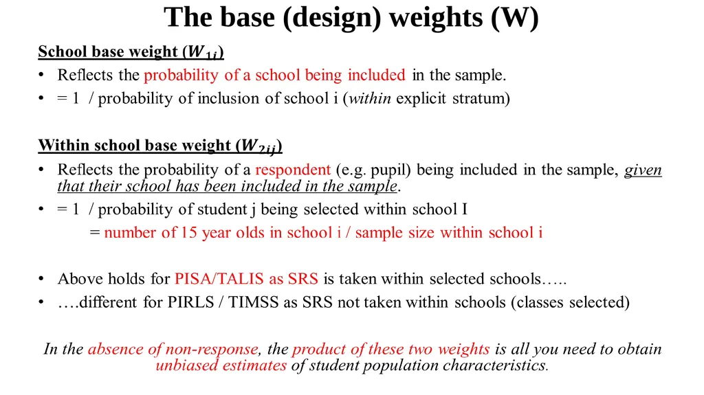
slide22. The base (design) weights (W)<br>
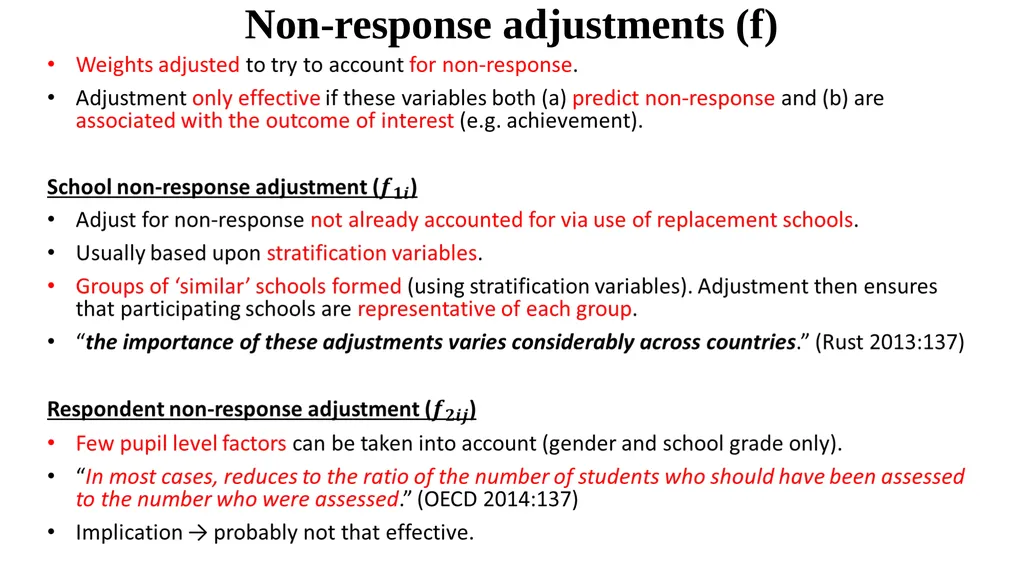
slide23. Non-response adjustments (f)<br>
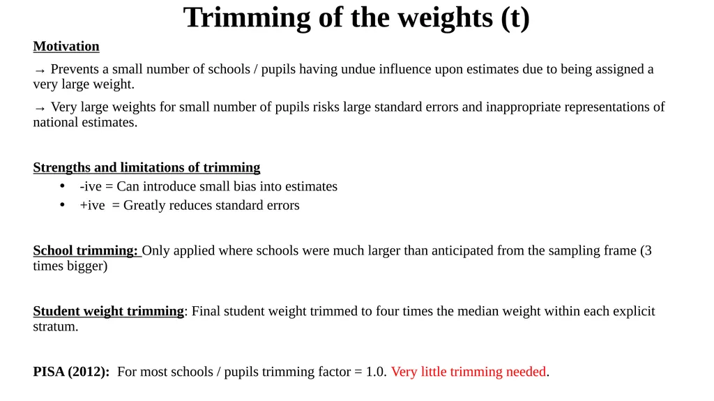
slide24. Trimming of the weights (t) Motivation
→ Prevents a small number of schools / pupils having undue influence upon estimates due to being assigned a very large weight.
→ Very large weights for small number of pupils risks large standard errors and inappropriate representations of national estimates.

Strengths and limitations of trimming
-ive = Can introduce small bias into estimates
+ive = Greatly reduces standard errors

School trimming: Only applied where schools were much larger than anticipated from the sampling frame (3 times bigger)

Student weight trimming: Final student weight trimmed to four times the median weight within each explicit stratum.

PISA (2012): For most schools / pupils trimming factor = 1.0. Very little trimming needed.<br>
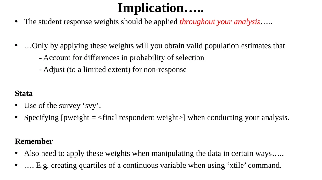
slide25. Implication….. The student response weights should be applied throughout your analysis…..

…Only by applying these weights will you obtain valid population estimates that
- Account for differences in probability of selection
- Adjust (to a limited extent) for non-response

Stata
Use of the survey ‘svy’.
Specifying [pweight = <final respondent weight>] when conducting your analysis.

Remember
Also need to apply these weights when manipulating the data in certain ways…..
…. E.g. creating quartiles of a continuous variable when using ‘xtile’ command.<br>
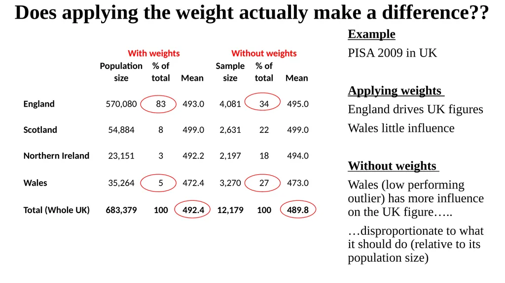
slide26. Does applying the weight actually make a difference?? Example
PISA 2009 in UK

Applying weights
England drives UK figures
Wales little influence

Without weights
Wales (low performing outlier) has more influence on the UK figure…..
…disproportionate to what it should do (relative to its population size)<br>
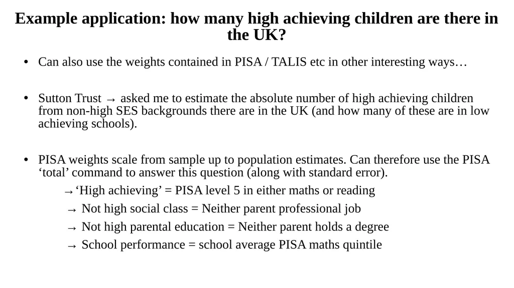
slide27. Example application: how many high achieving children are there in the UK? Can also use the weights contained in PISA / TALIS etc in other interesting ways…

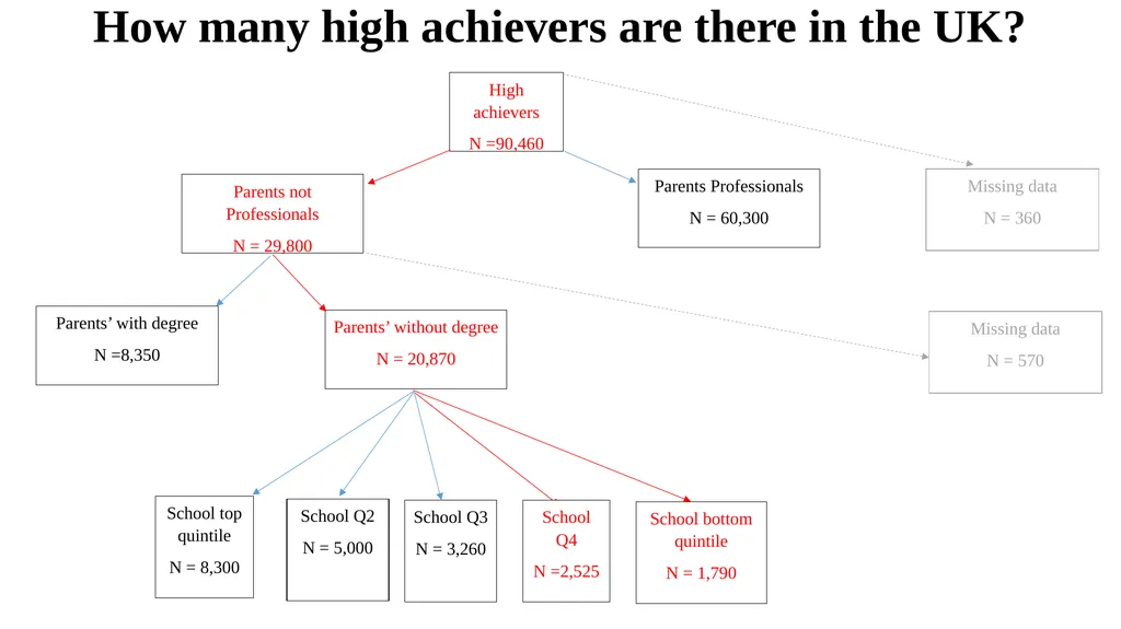
Sutton Trust → asked me to estimate the absolute number of high achieving children from non-high SES backgrounds there are in the UK (and how many of these are in low achieving schools).

PISA weights scale from sample up to population estimates. Can therefore use the PISA ‘total’ command to answer this question (along with standard error).
→‘High achieving’ = PISA level 5 in either maths or reading
→ Not high social class = Neither parent professional job
→ Not high parental education = Neither parent holds a degree
→ School performance = school average PISA maths quintile<br>
slide28. How many high achievers are there in the UK?<br>
slide29. Replication weights<br>
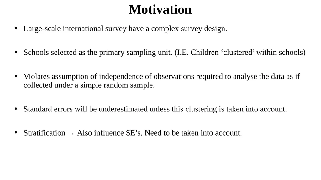
slide30. Motivation Large-scale international survey have a complex survey design.

Schools selected as the primary sampling unit. (I.E. Children ‘clustered’ within schools)

Violates assumption of independence of observations required to analyse the data as if collected under a simple random sample.

Standard errors will be underestimated unless this clustering is taken into account.

Stratification → Also influence SE’s. Need to be taken into account.<br>
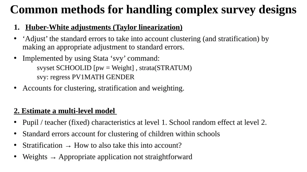
slide31. Common methods for handling complex survey designs Huber-White adjustments (Taylor linearization)
‘Adjust’ the standard errors to take into account clustering (and stratification) by making an appropriate adjustment to standard errors.
Implemented by using Stata ‘svy’ command:
svyset SCHOOLID [pw = Weight] , strata(STRATUM)
svy: regress PV1MATH GENDER
Accounts for clustering, stratification and weighting.

2. Estimate a multi-level model
Pupil / teacher (fixed) characteristics at level 1. School random effect at level 2.
Standard errors account for clustering of children within schools
Stratification → How to also take this into account?
Weights → Appropriate application not straightforward<br>
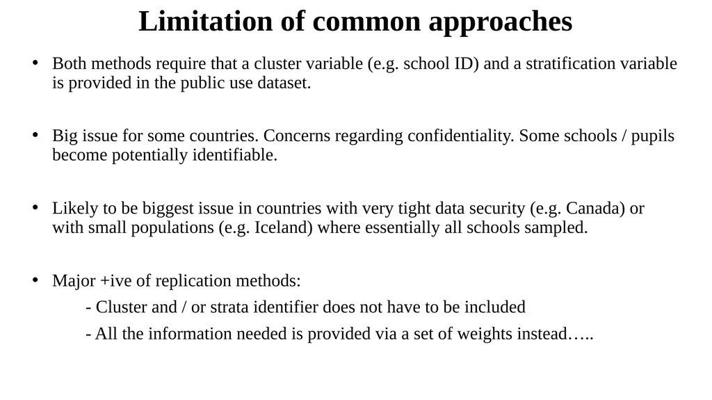
slide32. Limitation of common approaches Both methods require that a cluster variable (e.g. school ID) and a stratification variable is provided in the public use dataset.

Big issue for some countries. Concerns regarding confidentiality. Some schools / pupils become potentially identifiable.

Likely to be biggest issue in countries with very tight data security (e.g. Canada) or with small populations (e.g. Iceland) where essentially all schools sampled.

Major +ive of replication methods:
- Cluster and / or strata identifier does not have to be included
- All the information needed is provided via a set of weights instead…..<br>
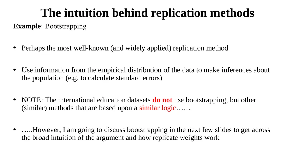
slide33. The intuition behind replication methods Example: Bootstrapping

Perhaps the most well-known (and widely applied) replication method

Use information from the empirical distribution of the data to make inferences about the population (e.g. to calculate standard errors)

NOTE: The international education datasets do not use bootstrapping, but other (similar) methods that are based upon a similar logic……

…..However, I am going to discuss bootstrapping in the next few slides to get across the broad intuition of the argument and how replicate weights work<br>
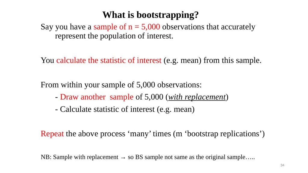
slide34. What is bootstrapping? Say you have a sample of n = 5,000 observations that accurately represent the population of interest.

You calculate the statistic of interest (e.g. mean) from this sample.

From within your sample of 5,000 observations:
- Draw another sample of 5,000 (with replacement)
- Calculate statistic of interest (e.g. mean)

Repeat the above process ‘many’ times (m ‘bootstrap replications’)

NB: Sample with replacement → so BS sample not same as the original sample….. 34<br>
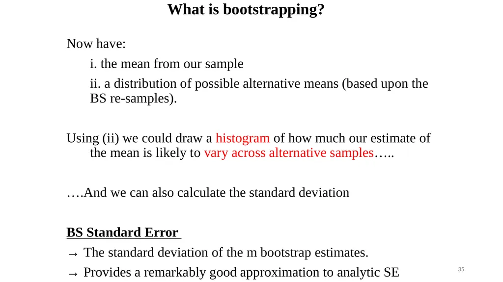
slide35. What is bootstrapping? Now have:
i. the mean from our sample
ii. a distribution of possible alternative means (based upon the BS re-samples).

Using (ii) we could draw a histogram of how much our estimate of the mean is likely to vary across alternative samples…..

….And we can also calculate the standard deviation

BS Standard Error
→ The standard deviation of the m bootstrap estimates.
→ Provides a remarkably good approximation to analytic SE 35<br>
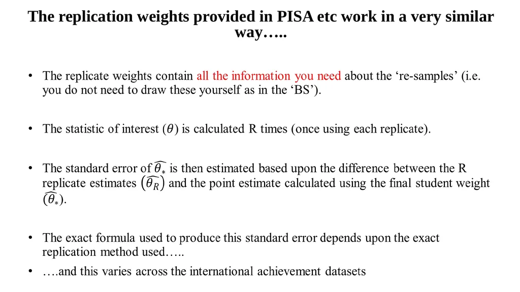
slide36. The replication weights provided in PISA etc work in a very similar way…..<br>
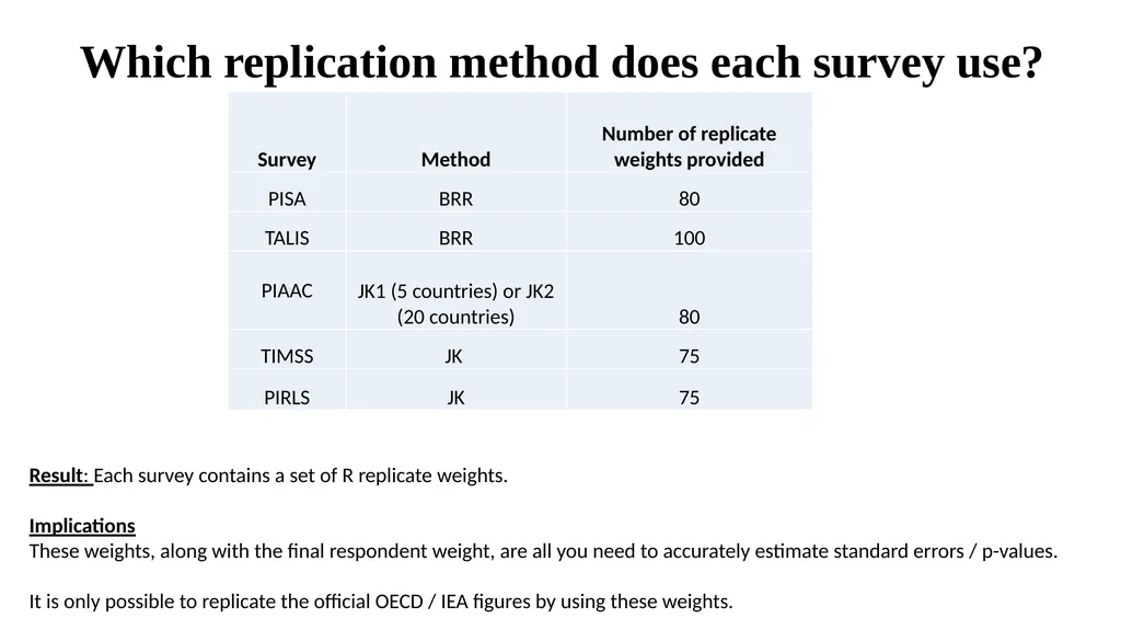
slide37. Which replication method does each survey use? Result: Each survey contains a set of R replicate weights.

Implications
These weights, along with the final respondent weight, are all you need to accurately estimate standard errors / p-values.

It is only possible to replicate the official OECD / IEA figures by using these weights.<br>
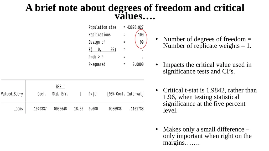
slide38. A brief note about degrees of freedom and critical values…. Number of degrees of freedom = Number of replicate weights – 1.

Impacts the critical value used in significance tests and CI’s.

Critical t-stat is 1.9842, rather than 1.96, when testing statistical significance at the five percent level.

Makes only a small difference – only important when right on the margins…….<br>
slide39. How do you use these replicate weights? See computer workshop providing examples using TALIS 2013 data!<br>
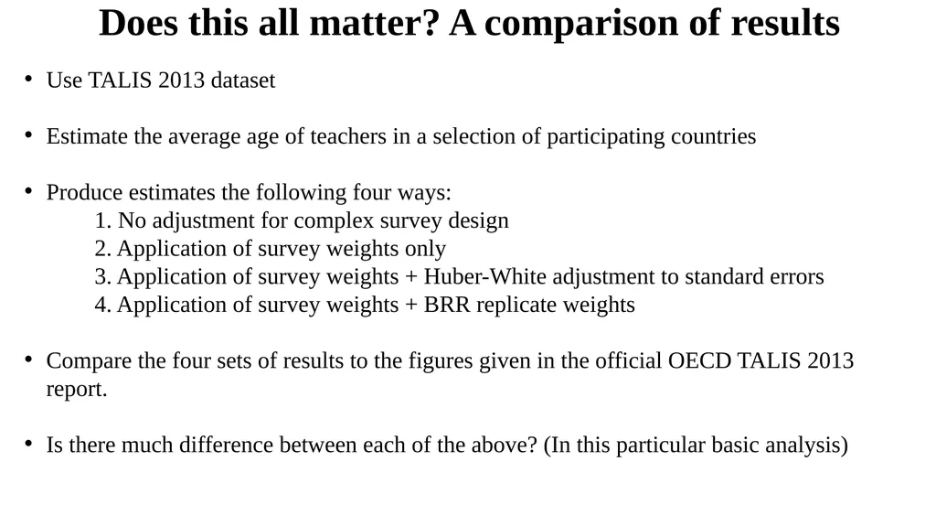
slide40. Does this all matter? A comparison of results Use TALIS 2013 dataset

Estimate the average age of teachers in a selection of participating countries

Produce estimates the following four ways:
1. No adjustment for complex survey design
2. Application of survey weights only
3. Application of survey weights + Huber-White adjustment to standard errors
4. Application of survey weights + BRR replicate weights

Compare the four sets of results to the figures given in the official OECD TALIS 2013 report.

Is there much difference between each of the above? (In this particular basic analysis)<br>
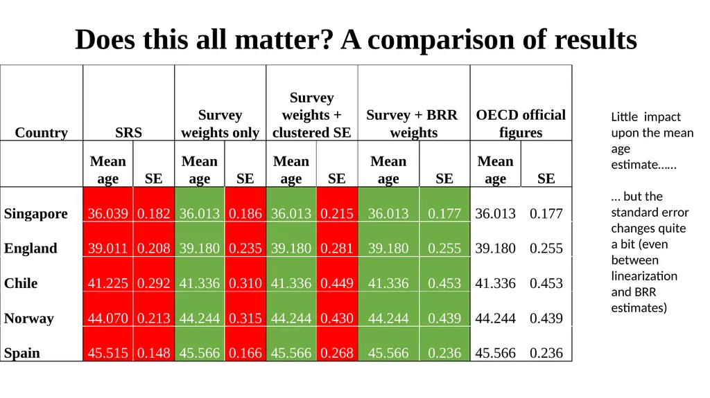
slide41. Does this all matter? A comparison of results Little impact upon the mean age estimate……

… but the standard error changes quite a bit (even between linearization and BRR estimates)<br>
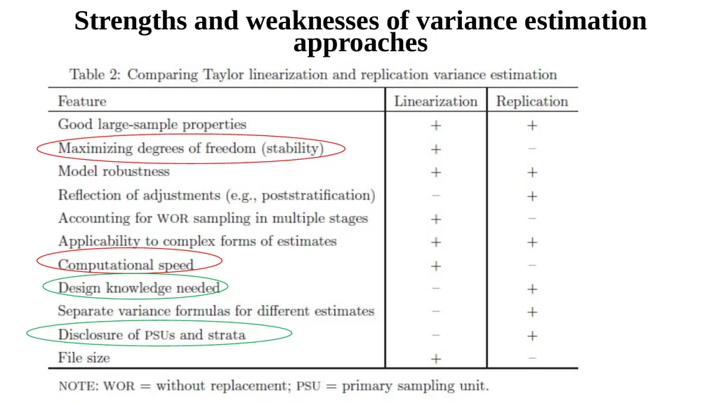
slide42. Strengths and weaknesses of variance estimation approaches<br>
slide43. Conclusions All of the international datasets use a complex survey design.

‘Strict’ criteria for response rates – though there is also some flexibility……

…..But OECD will chuck your country out if response rate really is too low

Survey weights incorporate complex design, non-response adjustment and (very limited) trimming.

Only by applying these weights will your point estimates be ‘correct’ (i.e. consistent estimates of population values)

Replication methods are used to estimate standard errors (and associated significance tests and confidence intervals)….

….Only by using these weights will you be able to replicate the OECD / IEA figures<br>