
VORTEX DYNAMICS OF CLASSICAL FLUIDS IN HIGHER
SN
Published · 40 slides · 0 views
1 / 1
Description
VORTEX DYNAMICS OF CLASSICAL FLUIDS IN HIGHER DIMENSIONS Banavara N. Shashikanth, Mechanical and Aerospace Engineering, New Mexico State University TexPoint fonts used in EMF. Read the TexPoint manual before you delete this box.:
Related Topics
Share
Embed code
Download this presentation From Below
"VORTEX DYNAMICS OF CLASSICAL FLUIDS IN HIGHER" is the property of its rightful owner. Permission is granted to download and print the materials on this website for personal, non-commercial use only, and to display it on your personal computer provided you do not modify the materials and that you retain all copyright notices contained in the materials. By downloading content from our website, you accept the terms of this agreement.
Presentation Transcript
01
VORTEX DYNAMICS OF CLASSICAL FLUIDS IN HIGHER DIMENSIONS Banavara N. Shashikanth,
Mechanical and Aerospace Engineering,
New Mexico State University TexPoint fonts used in EMF.
Read the TexPoint manual before you delete this box.: AAAAAAAAAAAAAAAAAAAA<br>
Mechanical and Aerospace Engineering,
New Mexico State University TexPoint fonts used in EMF.
Read the TexPoint manual before you delete this box.: AAAAAAAAAAAAAAAAAAAA<br>
02
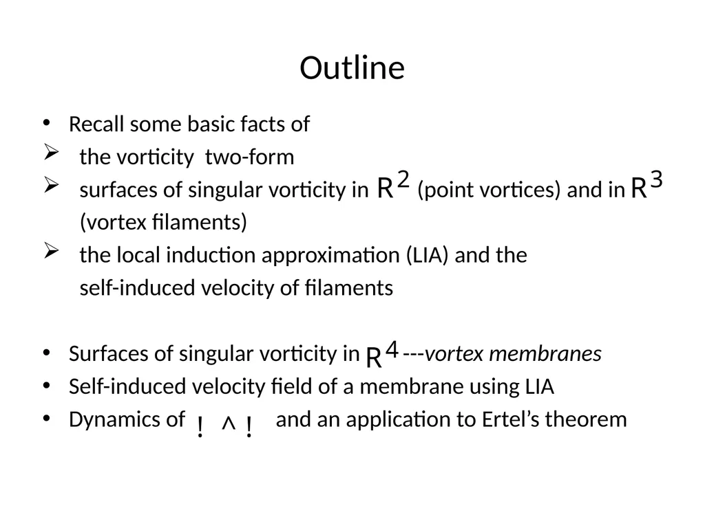
Outline Recall some basic facts of
the vorticity two-form
surfaces of singular vorticity in (point vortices) and in
(vortex filaments)
the local induction approximation (LIA) and the
self-induced velocity of filaments
Surfaces of singular vorticity in ---vortex membranes
Self-induced velocity field of a membrane using LIA
Dynamics of and an application to Ertel’s theorem<br>
the vorticity two-form
surfaces of singular vorticity in (point vortices) and in
(vortex filaments)
the local induction approximation (LIA) and the
self-induced velocity of filaments
Surfaces of singular vorticity in ---vortex membranes
Self-induced velocity field of a membrane using LIA
Dynamics of and an application to Ertel’s theorem<br>
03
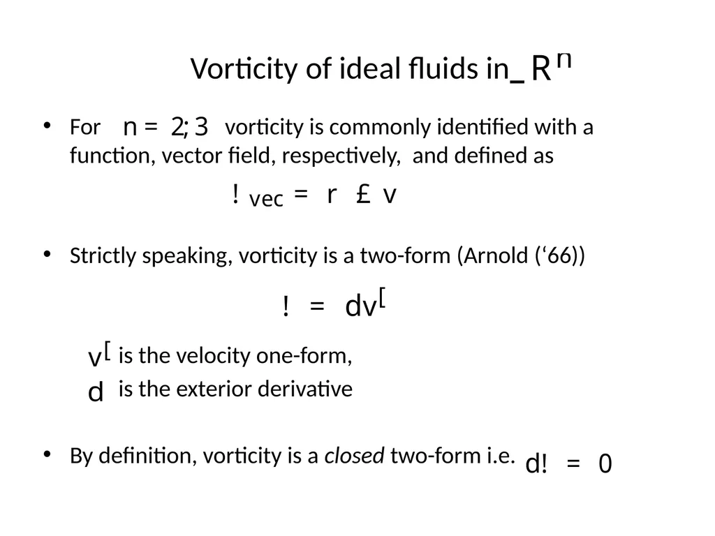
Vorticity of ideal fluids in For vorticity is commonly identified with a function, vector field, respectively, and defined as
Strictly speaking, vorticity is a two-form (Arnold (‘66))
is the velocity one-form,
is the exterior derivative
By definition, vorticity is a closed two-form i.e.<br>
Strictly speaking, vorticity is a two-form (Arnold (‘66))
is the velocity one-form,
is the exterior derivative
By definition, vorticity is a closed two-form i.e.<br>
04
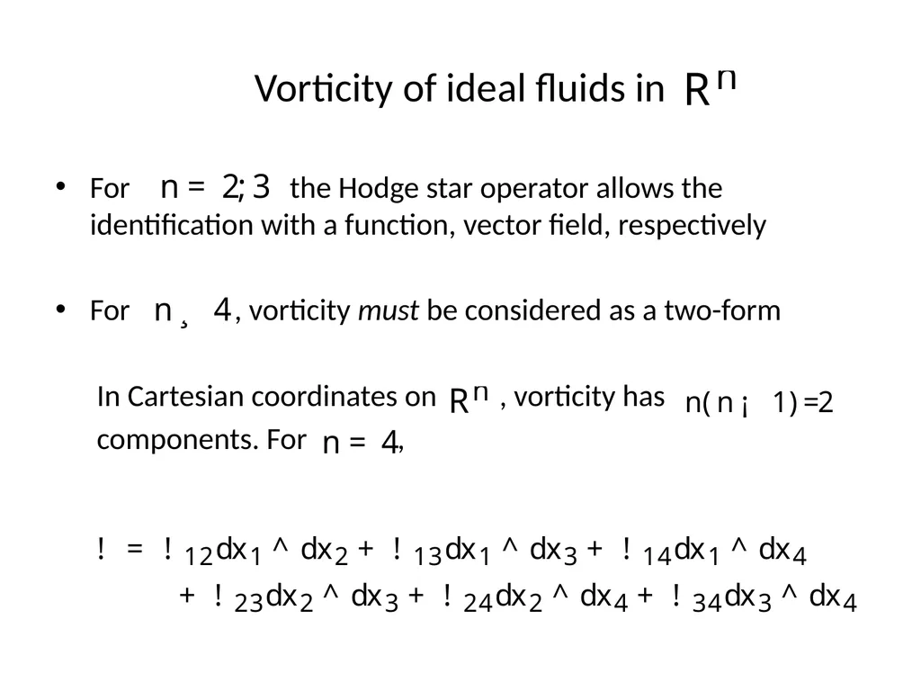
Vorticity of ideal fluids in For the Hodge star operator allows the identification with a function, vector field, respectively
For , vorticity must be considered as a two-form
In Cartesian coordinates on , vorticity has
components. For ,<br>
For , vorticity must be considered as a two-form
In Cartesian coordinates on , vorticity has
components. For ,<br>
05
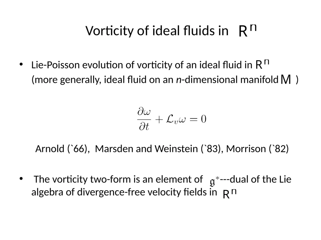
Vorticity of ideal fluids in Lie-Poisson evolution of vorticity of an ideal fluid in
(more generally, ideal fluid on an n-dimensional manifold )
Arnold (`66), Marsden and Weinstein (`83), Morrison (`82)
The vorticity two-form is an element of ---dual of the Lie algebra of divergence-free velocity fields in<br>
(more generally, ideal fluid on an n-dimensional manifold )
Arnold (`66), Marsden and Weinstein (`83), Morrison (`82)
The vorticity two-form is an element of ---dual of the Lie algebra of divergence-free velocity fields in<br>
06
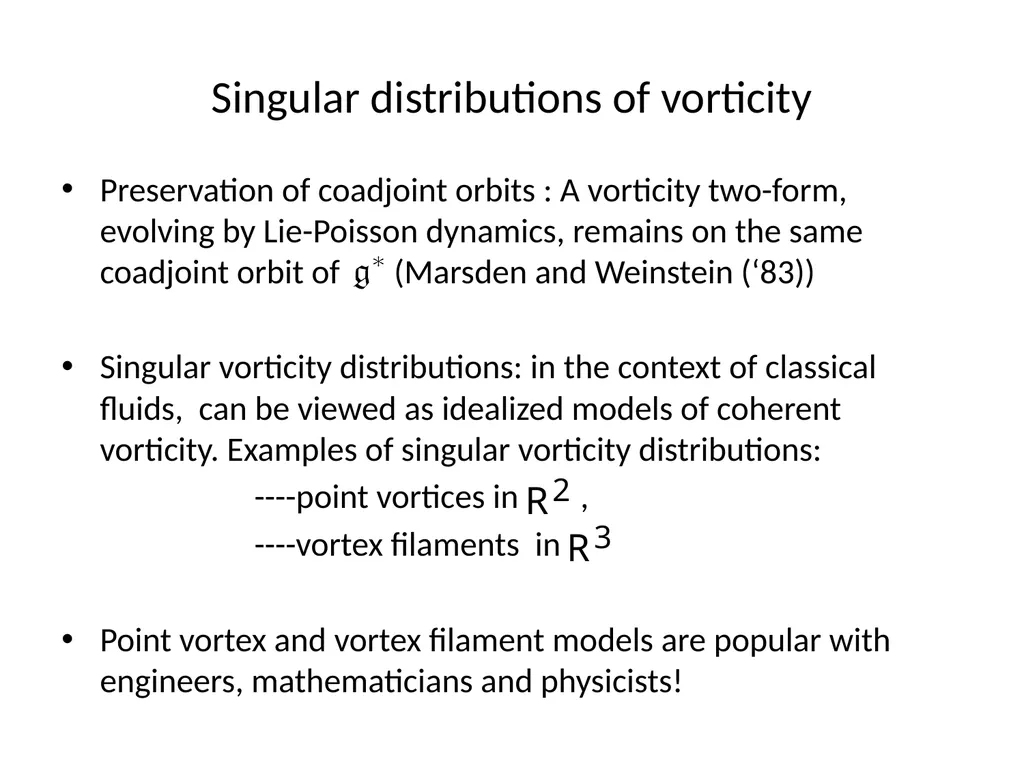
Singular distributions of vorticity Preservation of coadjoint orbits : A vorticity two-form, evolving by Lie-Poisson dynamics, remains on the same coadjoint orbit of (Marsden and Weinstein (‘83))
Singular vorticity distributions: in the context of classical fluids, can be viewed as idealized models of coherent vorticity. Examples of singular vorticity distributions:
----point vortices in ,
----vortex filaments in
Point vortex and vortex filament models are popular with engineers, mathematicians and physicists!<br>
Singular vorticity distributions: in the context of classical fluids, can be viewed as idealized models of coherent vorticity. Examples of singular vorticity distributions:
----point vortices in ,
----vortex filaments in
Point vortex and vortex filament models are popular with engineers, mathematicians and physicists!<br>
07
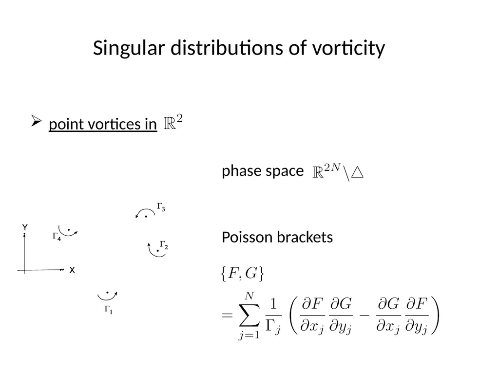
Singular distributions of vorticity point vortices in
phase space
Poisson brackets<br>
phase space
Poisson brackets<br>
08
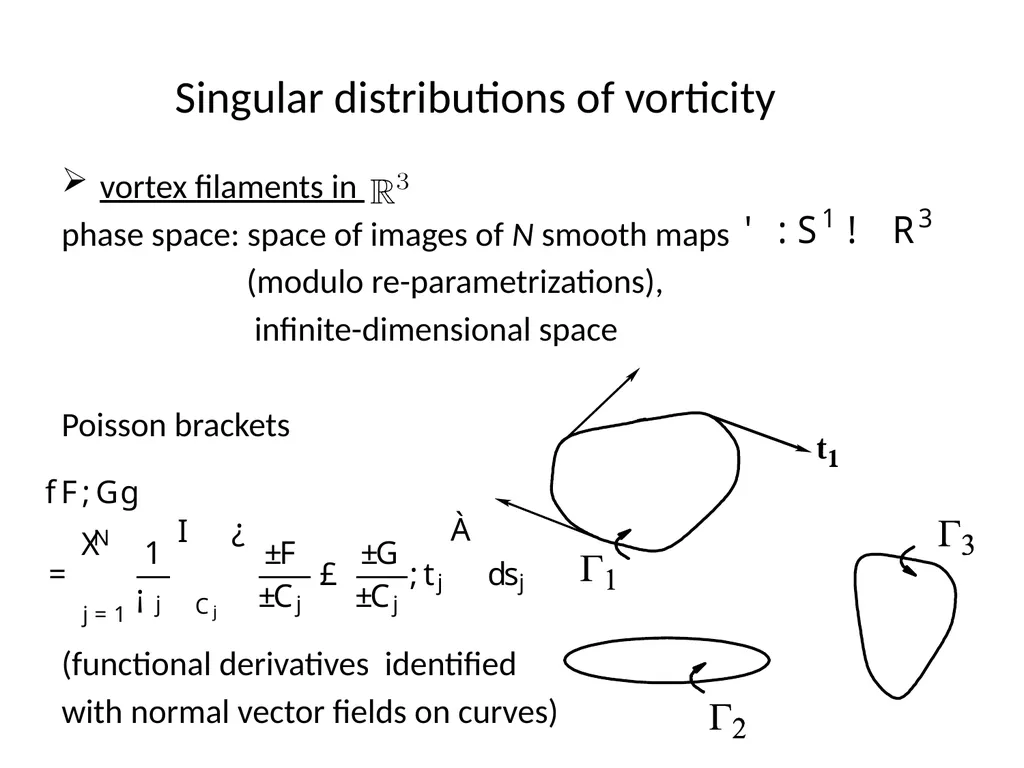
Singular distributions of vorticity vortex filaments in
phase space: space of images of N smooth maps
(modulo re-parametrizations),
infinite-dimensional space
Poisson brackets
(functional derivatives identified
with normal vector fields on curves)<br>
phase space: space of images of N smooth maps
(modulo re-parametrizations),
infinite-dimensional space
Poisson brackets
(functional derivatives identified
with normal vector fields on curves)<br>
09
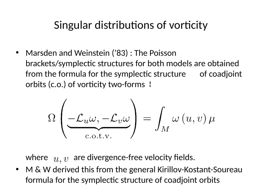
Singular distributions of vorticity Marsden and Weinstein (’83) : The Poisson brackets/symplectic structures for both models are obtained from the formula for the symplectic structure of coadjoint orbits (c.o.) of vorticity two-forms
where are divergence-free velocity fields.
M & W derived this from the general Kirillov-Kostant-Soureau formula for the symplectic structure of coadjoint orbits<br>
where are divergence-free velocity fields.
M & W derived this from the general Kirillov-Kostant-Soureau formula for the symplectic structure of coadjoint orbits<br>
10
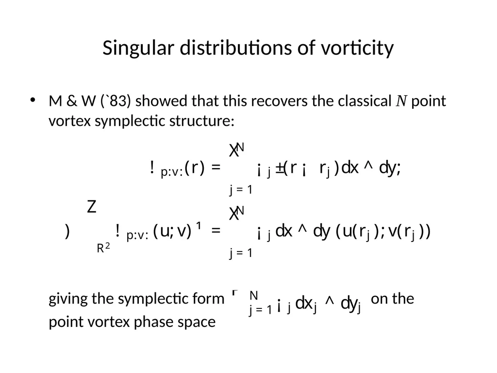
Singular distributions of vorticity M & W (`83) showed that this recovers the classical N point vortex symplectic structure:
giving the symplectic form on the
point vortex phase space<br>
giving the symplectic form on the
point vortex phase space<br>
11
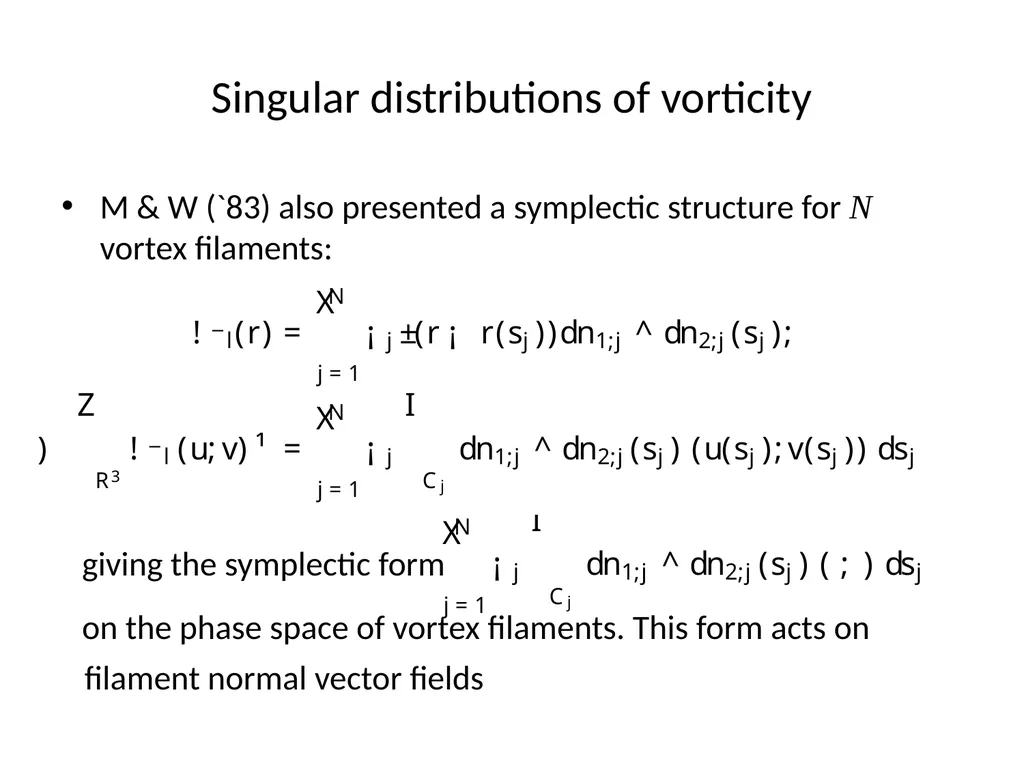
Singular distributions of vorticity M & W (`83) also presented a symplectic structure for N vortex filaments:
giving the symplectic form
on the phase space of vortex filaments. This form acts on
filament normal vector fields<br>
giving the symplectic form
on the phase space of vortex filaments. This form acts on
filament normal vector fields<br>
12
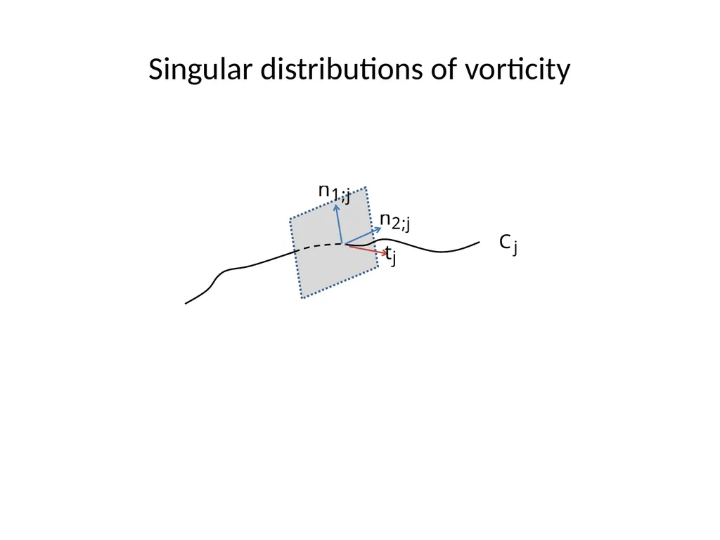
Singular distributions of vorticity<br>
13
Singular distributions of vorticity General geometric features of point vortices and vortex filaments:
They are co-dimension 2 surfaces
The vorticity two-form acts on planes that intersect these surfaces transversally. More precisely, the two-form is perpendicular to these surfaces.
Equivalently, using the Hodge star operator in , the n-2 form is tangent to these surfaces<br>
They are co-dimension 2 surfaces
The vorticity two-form acts on planes that intersect these surfaces transversally. More precisely, the two-form is perpendicular to these surfaces.
Equivalently, using the Hodge star operator in , the n-2 form is tangent to these surfaces<br>
14
Singular distributions of vorticity Minimum dimension of the surfaces
= the degree of the form
= n-2
Can we have singular distributions that do not satisfy the above?
For example, point vortices in or `vortons’
(Novikov (`83), Leonard (`85)). Here, each point is
also assigned a (time-varying) direction vector and
the `vorticity’ two-form acts on the single plane to which it is
normal. This `vorticity’ two-form is not closed i.e. !<br>
= the degree of the form
= n-2
Can we have singular distributions that do not satisfy the above?
For example, point vortices in or `vortons’
(Novikov (`83), Leonard (`85)). Here, each point is
also assigned a (time-varying) direction vector and
the `vorticity’ two-form acts on the single plane to which it is
normal. This `vorticity’ two-form is not closed i.e. !<br>
15
Singular distributions of vorticity Moving on to
We consider two-dimensional surfaces/manifolds to which
---now, a two-form---is tangent. We term these
surfaces vortex membranes
At each point of such a (co-dimension 2) surface there exists a plane of normals<br>
We consider two-dimensional surfaces/manifolds to which
---now, a two-form---is tangent. We term these
surfaces vortex membranes
At each point of such a (co-dimension 2) surface there exists a plane of normals<br>
16
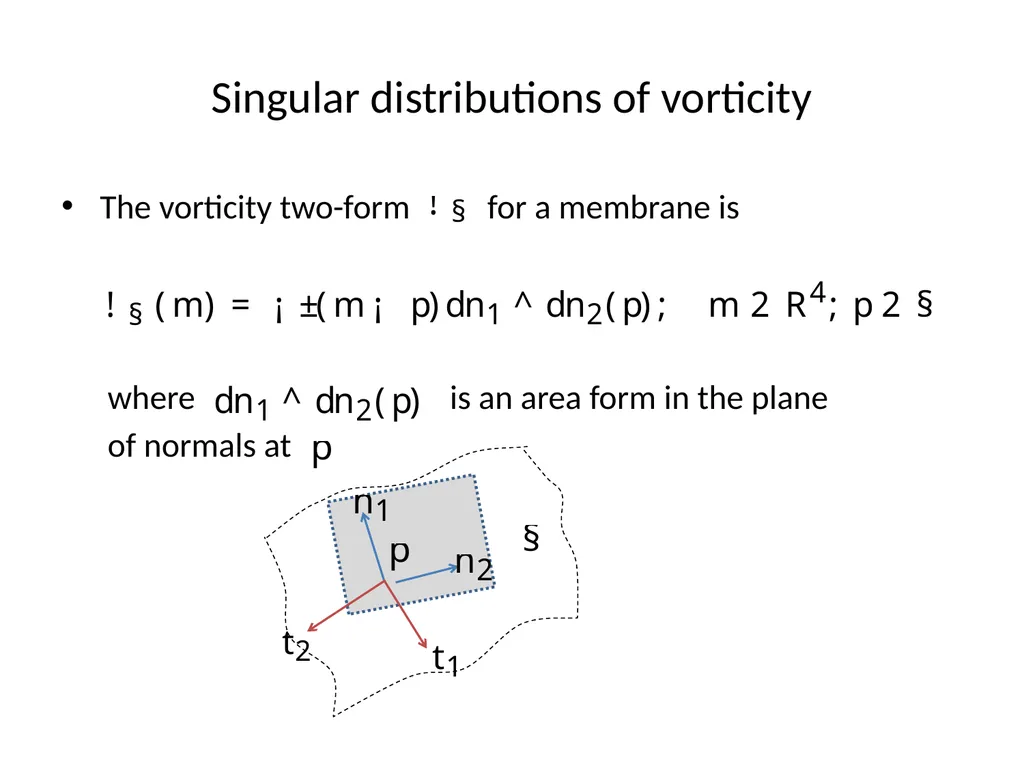
Singular distributions of vorticity The vorticity two-form for a membrane is
where is an area form in the plane
of normals at<br>
where is an area form in the plane
of normals at<br>
17
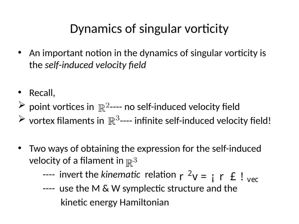
Dynamics of singular vorticity An important notion in the dynamics of singular vorticity is the self-induced velocity field
Recall,
point vortices in ---- no self-induced velocity field
vortex filaments in ---- infinite self-induced velocity field!
Two ways of obtaining the expression for the self-induced velocity of a filament in
---- invert the kinematic relation
---- use the M & W symplectic structure and the
kinetic energy Hamiltonian<br>
Recall,
point vortices in ---- no self-induced velocity field
vortex filaments in ---- infinite self-induced velocity field!
Two ways of obtaining the expression for the self-induced velocity of a filament in
---- invert the kinematic relation
---- use the M & W symplectic structure and the
kinetic energy Hamiltonian<br>
18
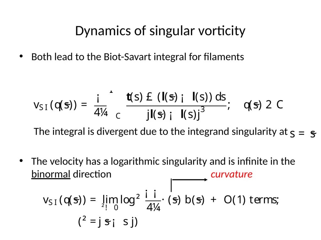
Dynamics of singular vorticity Both lead to the Biot-Savart integral for filaments
The integral is divergent due to the integrand singularity at
The velocity has a logarithmic singularity and is infinite in the binormal direction curvature<br>
The integral is divergent due to the integrand singularity at
The velocity has a logarithmic singularity and is infinite in the binormal direction curvature<br>
19
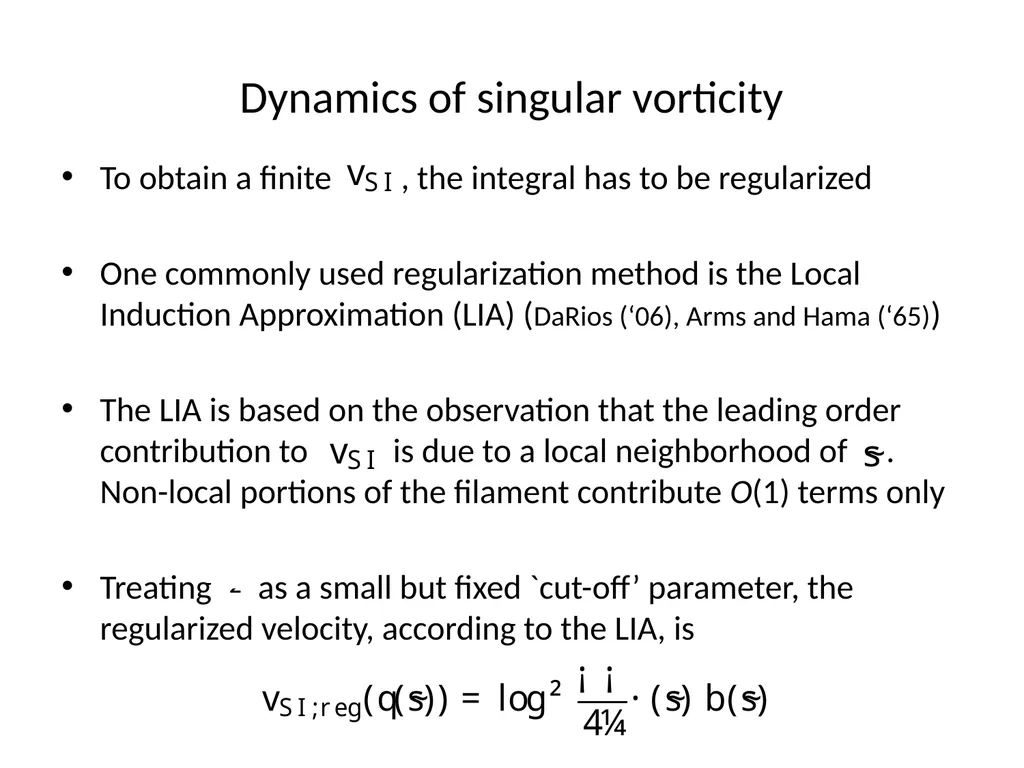
Dynamics of singular vorticity To obtain a finite , the integral has to be regularized
One commonly used regularization method is the Local Induction Approximation (LIA) (DaRios (‘06), Arms and Hama (‘65))
The LIA is based on the observation that the leading order contribution to is due to a local neighborhood of . Non-local portions of the filament contribute O(1) terms only
Treating as a small but fixed `cut-off’ parameter, the regularized velocity, according to the LIA, is<br>
One commonly used regularization method is the Local Induction Approximation (LIA) (DaRios (‘06), Arms and Hama (‘65))
The LIA is based on the observation that the leading order contribution to is due to a local neighborhood of . Non-local portions of the filament contribute O(1) terms only
Treating as a small but fixed `cut-off’ parameter, the regularized velocity, according to the LIA, is<br>
20
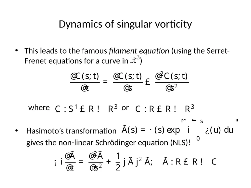
Dynamics of singular vorticity This leads to the famous filament equation (using the Serret-Frenet equations for a curve in )
where or
Hasimoto’s transformation
gives the non-linear Schrödinger equation (NLS)!<br>
where or
Hasimoto’s transformation
gives the non-linear Schrödinger equation (NLS)!<br>
21
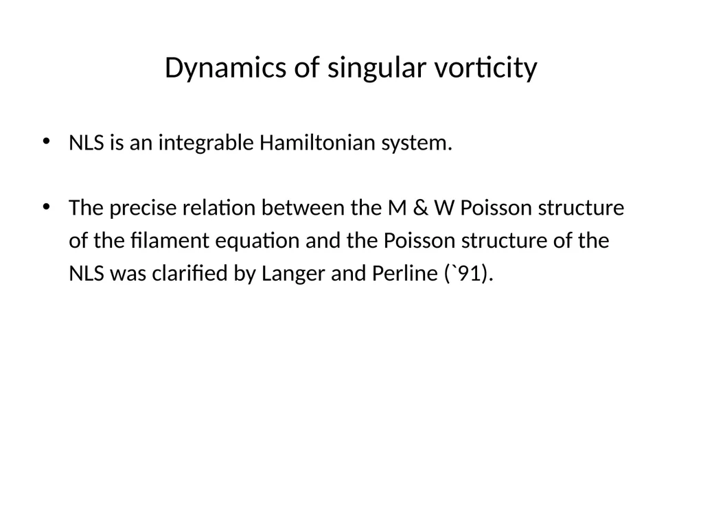
Dynamics of singular vorticity NLS is an integrable Hamiltonian system.
The precise relation between the M & W Poisson structure
of the filament equation and the Poisson structure of the
NLS was clarified by Langer and Perline (`91).<br>
The precise relation between the M & W Poisson structure
of the filament equation and the Poisson structure of the
NLS was clarified by Langer and Perline (`91).<br>
22
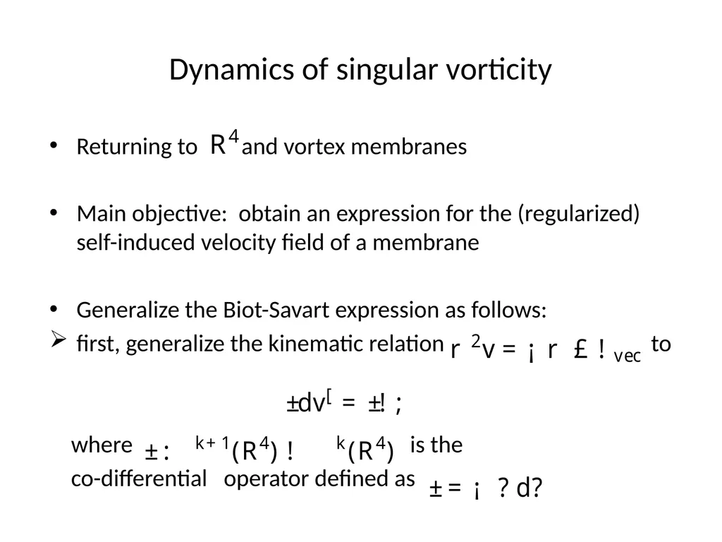
Dynamics of singular vorticity Returning to and vortex membranes
Main objective: obtain an expression for the (regularized) self-induced velocity field of a membrane
Generalize the Biot-Savart expression as follows:
first, generalize the kinematic relation to
where is the
co-differential operator defined as<br>
Main objective: obtain an expression for the (regularized) self-induced velocity field of a membrane
Generalize the Biot-Savart expression as follows:
first, generalize the kinematic relation to
where is the
co-differential operator defined as<br>
23
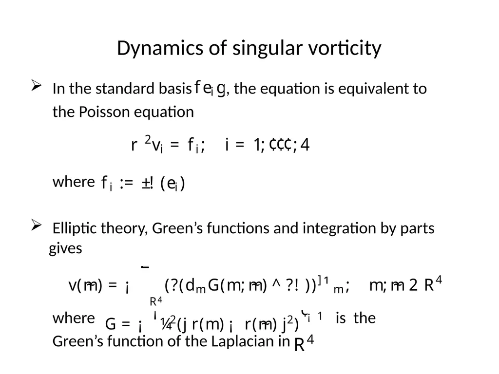
Dynamics of singular vorticity In the standard basis , the equation is equivalent to
the Poisson equation
where
Elliptic theory, Green’s functions and integration by parts gives
where is the
Green’s function of the Laplacian in<br>
the Poisson equation
where
Elliptic theory, Green’s functions and integration by parts gives
where is the
Green’s function of the Laplacian in<br>
24
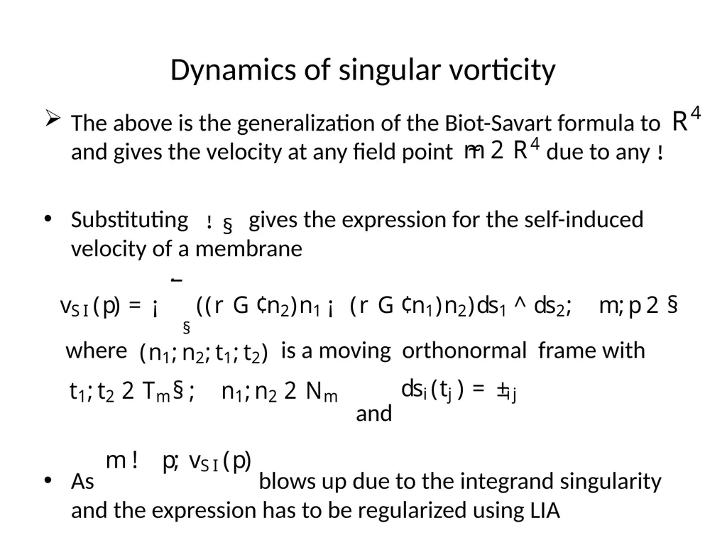
Dynamics of singular vorticity The above is the generalization of the Biot-Savart formula to and gives the velocity at any field point due to any
Substituting gives the expression for the self-induced velocity of a membrane
where is a moving orthonormal frame with
and
As blows up due to the integrand singularity and the expression has to be regularized using LIA<br>
Substituting gives the expression for the self-induced velocity of a membrane
where is a moving orthonormal frame with
and
As blows up due to the integrand singularity and the expression has to be regularized using LIA<br>
25
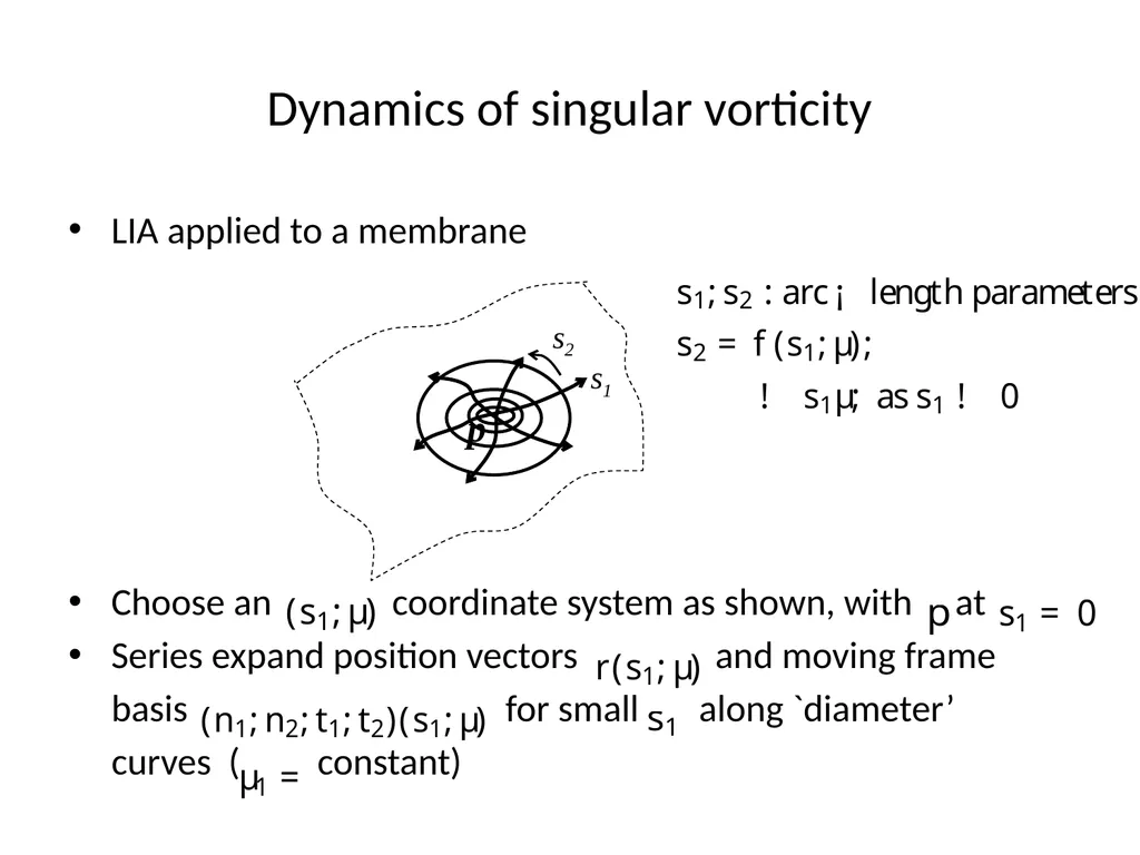
Dynamics of singular vorticity LIA applied to a membrane
Choose an coordinate system as shown, with at
Series expand position vectors and moving frame
basis for small along `diameter’
curves ( constant) s1 s2 p<br>
Choose an coordinate system as shown, with at
Series expand position vectors and moving frame
basis for small along `diameter’
curves ( constant) s1 s2 p<br>
26
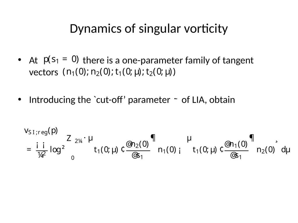
Dynamics of singular vorticity At there is a one-parameter family of tangent vectors
Introducing the `cut-off’ parameter of LIA, obtain<br>
Introducing the `cut-off’ parameter of LIA, obtain<br>
27
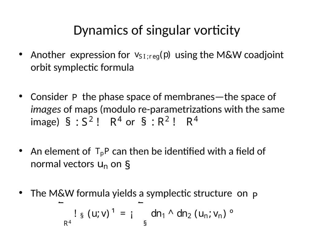
Dynamics of singular vorticity Another expression for using the M&W coadjoint orbit symplectic formula
Consider the phase space of membranes—the space of images of maps (modulo re-parametrizations with the same image) or
An element of can then be identified with a field of normal vectors on
The M&W formula yields a symplectic structure on<br>
Consider the phase space of membranes—the space of images of maps (modulo re-parametrizations with the same image) or
An element of can then be identified with a field of normal vectors on
The M&W formula yields a symplectic structure on<br>
28
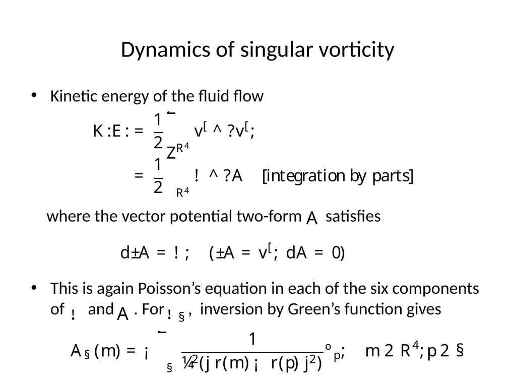
Dynamics of singular vorticity Kinetic energy of the fluid flow
where the vector potential two-form satisfies
This is again Poisson’s equation in each of the six components of and . For , inversion by Green’s function gives<br>
where the vector potential two-form satisfies
This is again Poisson’s equation in each of the six components of and . For , inversion by Green’s function gives<br>
29
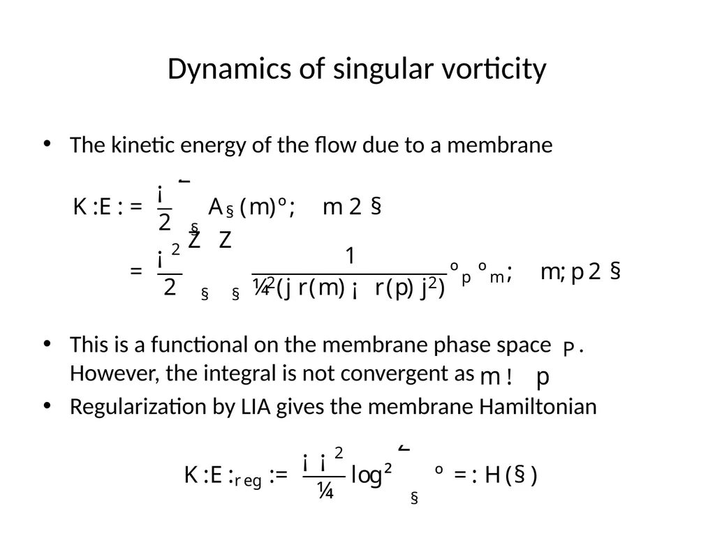
Dynamics of singular vorticity The kinetic energy of the flow due to a membrane
This is a functional on the membrane phase space . However, the integral is not convergent as
Regularization by LIA gives the membrane Hamiltonian<br>
This is a functional on the membrane phase space . However, the integral is not convergent as
Regularization by LIA gives the membrane Hamiltonian<br>
30
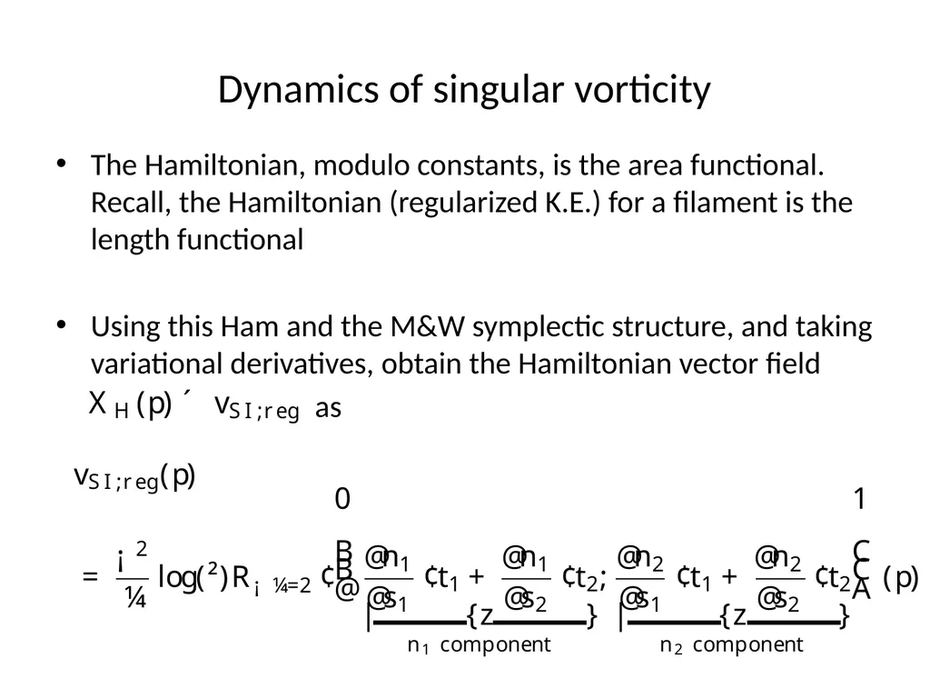
Dynamics of singular vorticity The Hamiltonian, modulo constants, is the area functional. Recall, the Hamiltonian (regularized K.E.) for a filament is the length functional
Using this Ham and the M&W symplectic structure, and taking variational derivatives, obtain the Hamiltonian vector field
as<br>
Using this Ham and the M&W symplectic structure, and taking variational derivatives, obtain the Hamiltonian vector field
as<br>
31
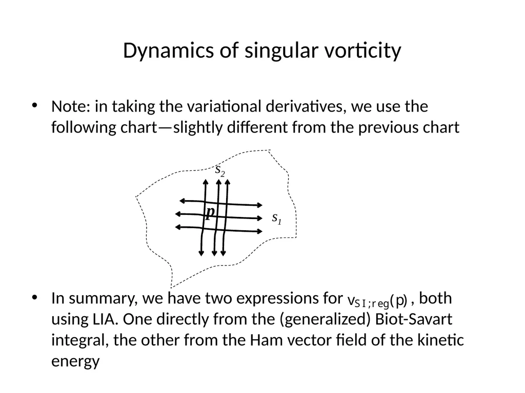
Dynamics of singular vorticity Note: in taking the variational derivatives, we use the following chart—slightly different from the previous chart
In summary, we have two expressions for , both using LIA. One directly from the (generalized) Biot-Savart integral, the other from the Ham vector field of the kinetic energy s1 s2 p<br>
In summary, we have two expressions for , both using LIA. One directly from the (generalized) Biot-Savart integral, the other from the Ham vector field of the kinetic energy s1 s2 p<br>
32
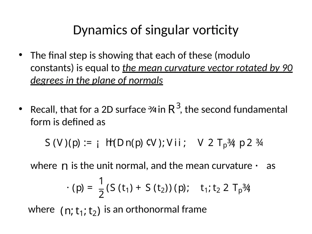
Dynamics of singular vorticity The final step is showing that each of these (modulo constants) is equal to the mean curvature vector rotated by 90 degrees in the plane of normals
Recall, that for a 2D surface in , the second fundamental form is defined as
where is the unit normal, and the mean curvature as
where is an orthonormal frame<br>
Recall, that for a 2D surface in , the second fundamental form is defined as
where is the unit normal, and the mean curvature as
where is an orthonormal frame<br>
33
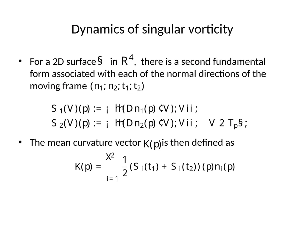
Dynamics of singular vorticity For a 2D surface in , there is a second fundamental form associated with each of the normal directions of the moving frame
The mean curvature vector is then defined as<br>
The mean curvature vector is then defined as<br>
34
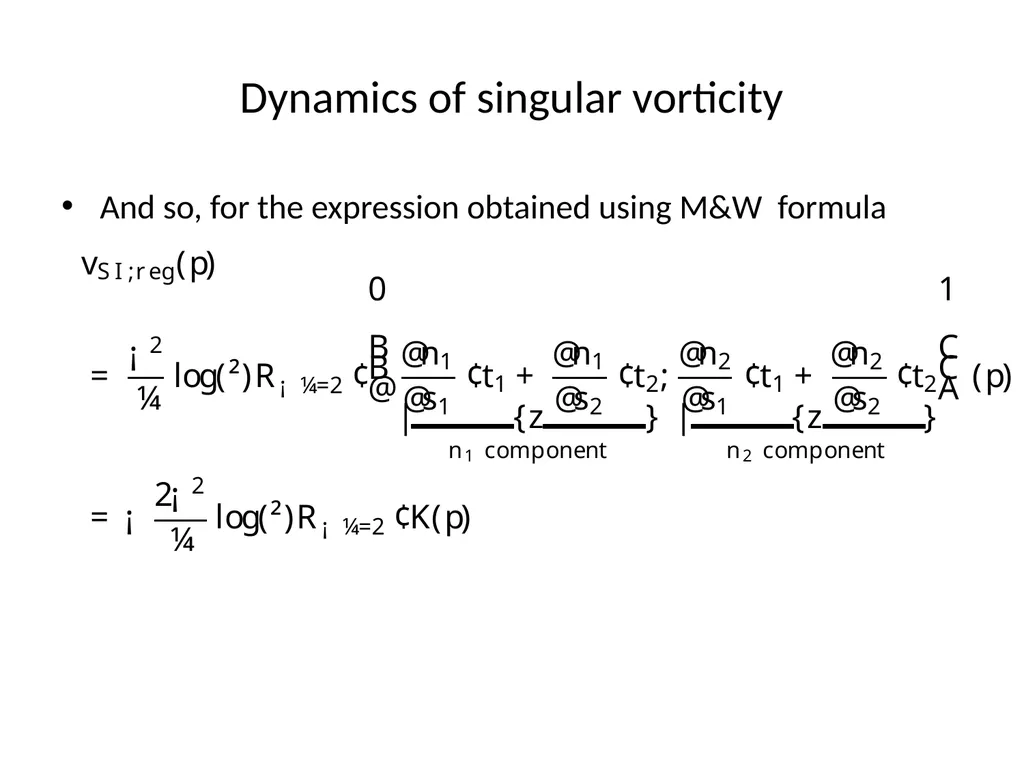
Dynamics of singular vorticity And so, for the expression obtained using M&W formula<br>
35
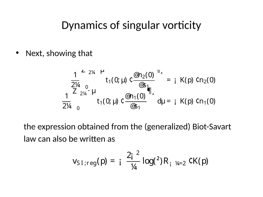
Dynamics of singular vorticity Next, showing that
the expression obtained from the (generalized) Biot-Savart
law can also be written as<br>
the expression obtained from the (generalized) Biot-Savart
law can also be written as<br>
36
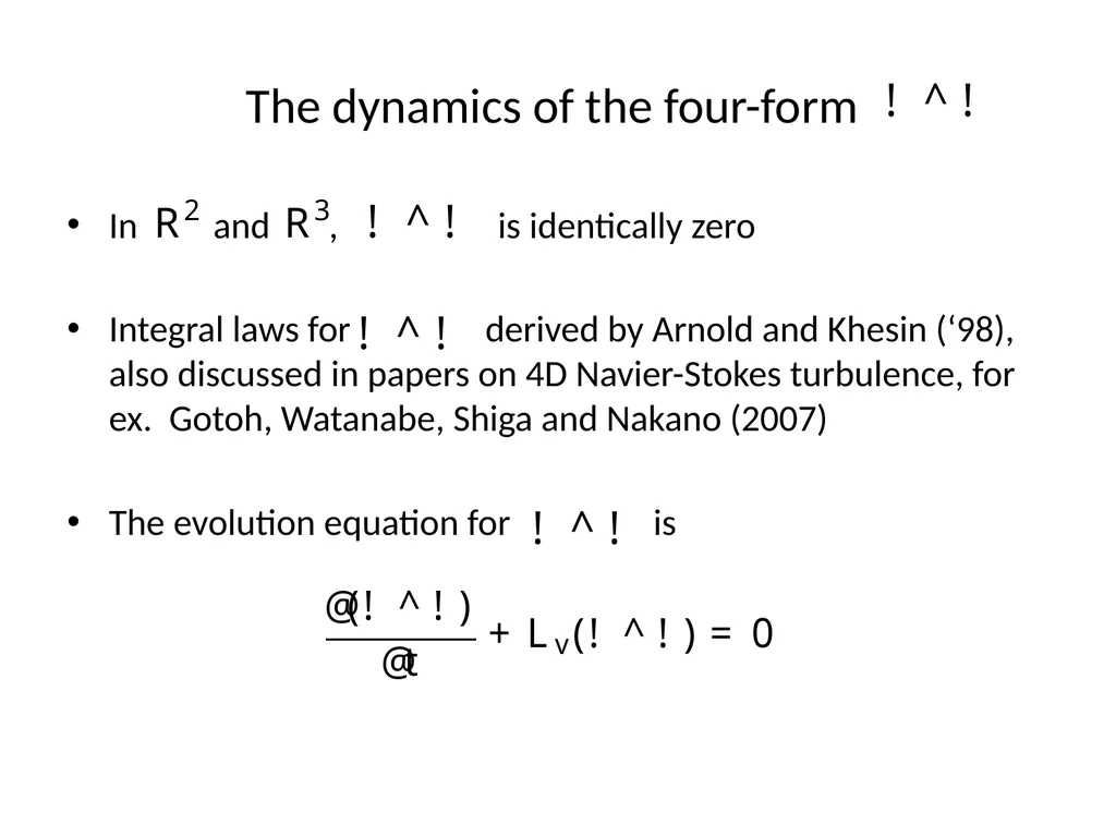
The dynamics of the four-form In and , is identically zero
Integral laws for derived by Arnold and Khesin (‘98), also discussed in papers on 4D Navier-Stokes turbulence, for ex. Gotoh, Watanabe, Shiga and Nakano (2007)
The evolution equation for is<br>
Integral laws for derived by Arnold and Khesin (‘98), also discussed in papers on 4D Navier-Stokes turbulence, for ex. Gotoh, Watanabe, Shiga and Nakano (2007)
The evolution equation for is<br>
37
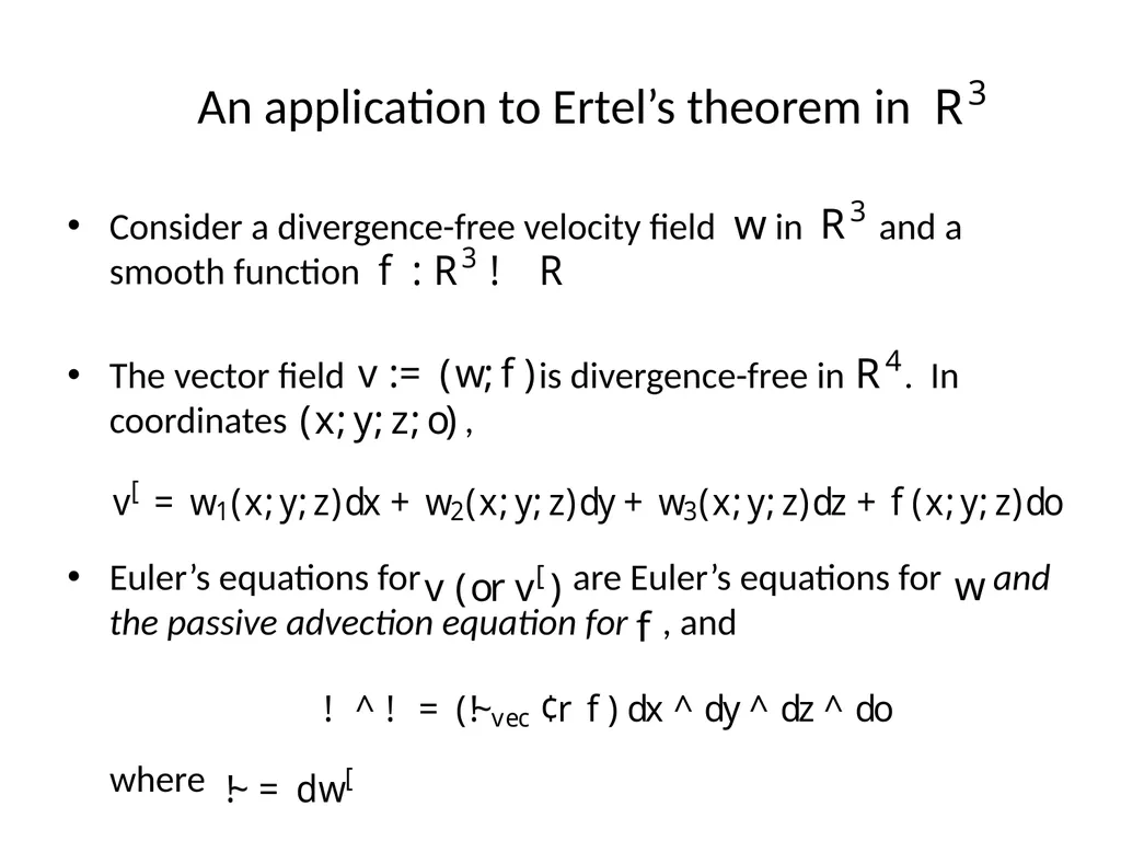
An application to Ertel’s theorem in Consider a divergence-free velocity field in and a smooth function
The vector field is divergence-free in . In coordinates ,
Euler’s equations for are Euler’s equations for and the passive advection equation for , and
where<br>
The vector field is divergence-free in . In coordinates ,
Euler’s equations for are Euler’s equations for and the passive advection equation for , and
where<br>
38
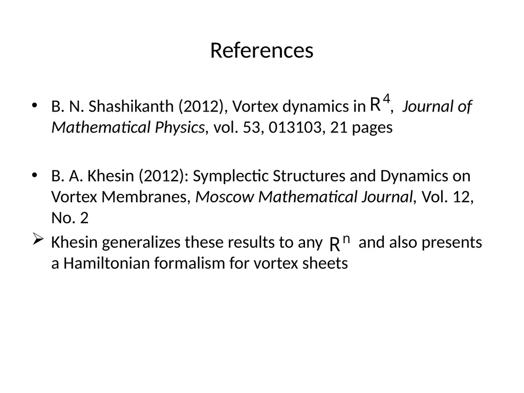
References B. N. Shashikanth (2012), Vortex dynamics in , Journal of Mathematical Physics, vol. 53, 013103, 21 pages
B. A. Khesin (2012): Symplectic Structures and Dynamics on Vortex Membranes, Moscow Mathematical Journal, Vol. 12, No. 2
Khesin generalizes these results to any and also presents a Hamiltonian formalism for vortex sheets<br>
B. A. Khesin (2012): Symplectic Structures and Dynamics on Vortex Membranes, Moscow Mathematical Journal, Vol. 12, No. 2
Khesin generalizes these results to any and also presents a Hamiltonian formalism for vortex sheets<br>
39
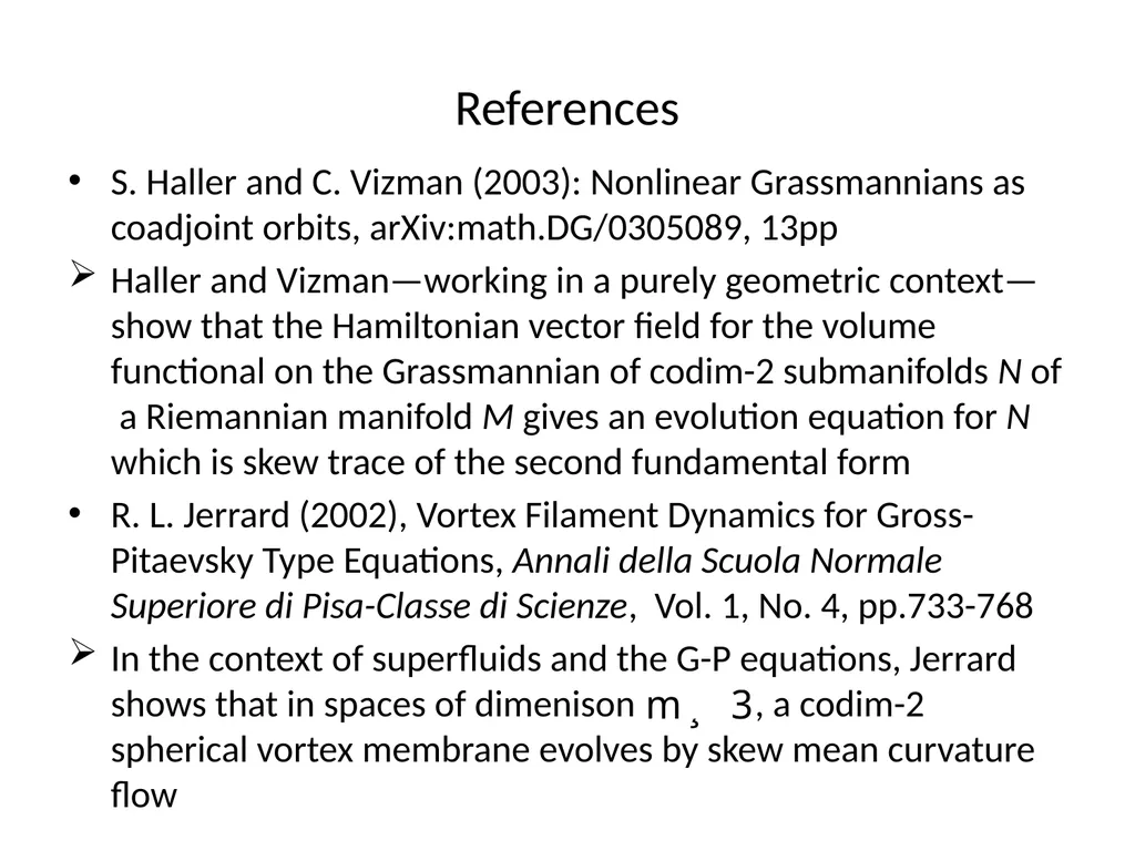
References S. Haller and C. Vizman (2003): Nonlinear Grassmannians as coadjoint orbits, arXiv:math.DG/0305089, 13pp
Haller and Vizman—working in a purely geometric context—show that the Hamiltonian vector field for the volume functional on the Grassmannian of codim-2 submanifolds N of a Riemannian manifold M gives an evolution equation for N which is skew trace of the second fundamental form
R. L. Jerrard (2002), Vortex Filament Dynamics for Gross-Pitaevsky Type Equations, Annali della Scuola Normale Superiore di Pisa-Classe di Scienze, Vol. 1, No. 4, pp.733-768
In the context of superfluids and the G-P equations, Jerrard shows that in spaces of dimenison , a codim-2 spherical vortex membrane evolves by skew mean curvature flow<br>
Haller and Vizman—working in a purely geometric context—show that the Hamiltonian vector field for the volume functional on the Grassmannian of codim-2 submanifolds N of a Riemannian manifold M gives an evolution equation for N which is skew trace of the second fundamental form
R. L. Jerrard (2002), Vortex Filament Dynamics for Gross-Pitaevsky Type Equations, Annali della Scuola Normale Superiore di Pisa-Classe di Scienze, Vol. 1, No. 4, pp.733-768
In the context of superfluids and the G-P equations, Jerrard shows that in spaces of dimenison , a codim-2 spherical vortex membrane evolves by skew mean curvature flow<br>
40
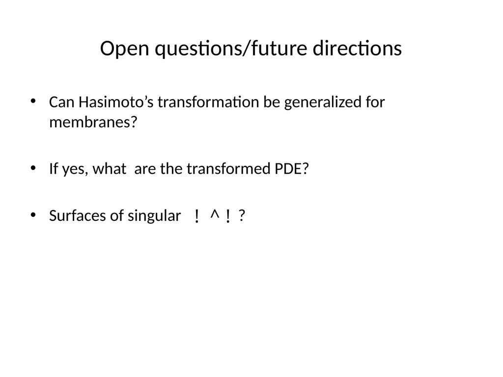
Open questions/future directions Can Hasimoto’s transformation be generalized for membranes?
If yes, what are the transformed PDE?
Surfaces of singular ?<br>
If yes, what are the transformed PDE?
Surfaces of singular ?<br>