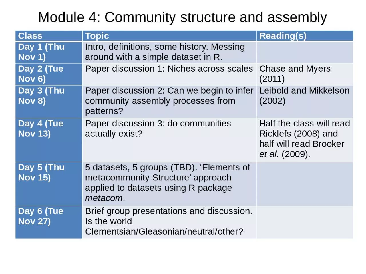
Class Topic Readings Day 1 Thu Nov 1 Intro definitions some history Messing around with a simple dataset in R Day 2 Tue Nov 6 Paper discussion 1 Niches across scales Chase and Myers 2011 ID: 1020019
Download Presentation The PPT/PDF document "Module 4: Community structure and asse..." is the property of its rightful owner. Permission is granted to download and print the materials on this web site for personal, non-commercial use only, and to display it on your personal computer provided you do not modify the materials and that you retain all copyright notices contained in the materials. By downloading content from our website, you accept the terms of this agreement.
1. Module 4: Community structure and assemblyClassTopicReading(s)Day 1 (Thu Nov 1)Intro, definitions, some history. Messing around with a simple dataset in R. Day 2 (Tue Nov 6)Paper discussion 1: Niches across scalesChase and Myers (2011)Day 3 (Thu Nov 8)Paper discussion 2: Can we begin to infer community assembly processes from patterns?Leibold and Mikkelson (2002)Day 4 (Tue Nov 13)Paper discussion 3: do communities actually exist?Half the class will read Ricklefs (2008) and half will read Brooker et al. (2009).Day 5 (Thu Nov 15)5 datasets, 5 groups (TBD). ‘Elements of metacommunity Structure’ approach applied to datasets using R package metacom. Day 6 (Tue Nov 27)Brief group presentations and discussion. Is the world Clementsian/Gleasonian/neutral/other?
2. Themes of this moduleHow do we quantify diversity across scales?What does it tell us about community assembly?
3. Learning objectivesUnderstand key foundational ecological conceptsUnderstand some of the key mechanisms driving community assembly and patterns of diversity across scalesLearn basic R tools for analyzing communities and metacommunitiesWhat is the relationship between pattern and process, and what are limits to this relationship?
4. Some key conceptsThe nicheEnvironmental filteringCompetition and competitive exclusionSuccessionDispersal limitationCommunity assemblyMetacommunityDeterministic vs. stochastic processesNiche vs. neutral processes
5. NICHES
6. The niche concepthttps://www.merriam-webster.com
7. Grinnellian niche (Grinnell 1917)Eltonian niche (Elton 1927)Niche is “n-dimensional”, maps population dynamics onto environmental space (Hutchinson 1957)Competitive exclusion principle (Hardin 1960)MacArthur and Levins (1967): limiting similarityThe niche concept and competition
8. PrecipitationSpring temperatureModified from Clark et al. (2011)Red oakBeechHutchinson (1957): fundamental niche conceptTradeoff axisSpecies turnover occurs across this axis
9. PrecipitationSpring temperatureModified from Clark et al. (2011)Red oakBeechHutchinson (1957): fundamental niche conceptThe two species can co-occur in this parameter space, and compete for resources
10. PrecipitationSpring temperatureHutchinson (1957): fundamental niche conceptNo turnover in this case; there is nestedness across spaceSp ASp BSp CWhy doesn’t Sp C occur here? Biotic interaction with Sp A or B or ‘environmental filtering?’Fundamental vs. realized niche
11. Species distributions form successive Gaussian envelopes along environmental gradientsWhittaker (1965, 1967)Environmental gradient ABCD
12. COMPETITION
13. Resource consumption often leads to resource depletion – AND COMPETITIONThe ability of a species to maintain itself in a community is determined by the limiting resource level (R*) that results in zero net population growth (ZNPG).This depends on the supply and consumption rates of the resource and the reproduction and mortality rates of the consumer species.Tilman (1980); Tilman et al. (1981)Image/fig from Cain et al. (2014)
14. Two species may have different R* values corresponding to their respective ZNPG statesImage/fig from Cain et al. (2014)
15. In competition, Synedra has a lower R*, and outcompetes AsterionellaR* represents the level of the resource that will allow a species to persistIf R* is low, the resource is being used efficientlyWhat can we say about the niches of each of these species? Image/fig from Cain et al. (2014)
16. http://corn.osu.edu/von Liebig's Law of the Minimum: yield is proportional to the amount of the most limiting nutrient in the soilA population will grow until one resource becomes limiting for further growthOrganisms need many resources – but von Liebig suggested that at any given time only one is limitingWhat happens when there are multiple resources?Image/fig from Cain et al. (2014)
17. LOCAL COEXISTENCE
18. Tilman’s R* provides a mechanism for understanding competitive exclusion and coexistence in terms of population dynamicsSpecies ASpecies BmAmBResource RR*BR*AGrowth rateTwo species, one resource – who wins?What happens when there are two potentially limiting resources?
19. Resource 1Resource 2Two species, two resourcesSpecies ASpecies BSpecies ASpecies BConsumption vectors123456Only a resource supply in zone 4 will lead to the coexistence point, but this shows that conditions exist that allow coexistence
20. Tilman showed experimentally that certain combinations of resource ratios and nutrient supply rates allowed stable coexistence between two diatom speciesImage/fig from Cain et al. (2014)
21. All plants need similar resources – how do so many species coexist?
22. At any given point in space, two species that don’t occupy the same niche can coexist when there are two limiting resourcesIt follows that if there are n limiting resources, n species can theoretically coexistBUT – there are only so many resources…Hutchinson (1961), in “The paradox of the plankton” asked, how do n+ species coexist on n resources?
23. Tilman (1988) expanded the two-species case to incorporate many species
24. One way -> if there is spatial variation in resource supply ratesIf the environment is homogeneous, we can think of the supply point as exactly that – a point, and only two species coexist Tilman (1988)
25. But if we have substantial spatial heterogeneity in supply rates and resource ratios, many species can coexistTilman (1988)
26. Another example: soil N and P in Barro Colorado Island (BCI), Panamahttp://www.life.illinois.edu/Soil NSoil P
27. MacArthur (1967)Myrtle warblerBlack-throated green warblerMacarthur’s warblers and niche partitioning
28.
29. To sum up: some mechanisms that may explain local species richness:Resource ratiosHutchinson (1961): Non-equilibriumSpatial heterogeneity in resource ratiosNiche partitioningOthers?
30. SUCCESSION
31. Clementsian vs. Gleasonian successionCowles (1899) -> succession in Lake Michigan dune communitiesClements (1916) -> communities as “super-organisms”, succession as analogous to development – climax stateGleason (1926) -> “individualistic model”: species interact during succession, but not in an integrated fashion
32. Horn (1975) and the Institute WoodsHorn (1975)
33. SassafrasRed mapleBeechHorn’s table in cartoon form…
34. A simulation of succession based on Horn’s overstory/understory data
35. Models of succession (Connel and Slatyer 1977)Disturbance creates colonization opportunitiesFacilitation: first species change conditions to allow later species to colonize. Implies high level of community integration. Inhibition: early-successional species inhibit colonization by all others. Late successional species are those that are able to survive better.Tolerance: later species take time to disperse, grow, and establish. They grow despite the presence of early-successional species, and eventually out-compete them.Climax
36. Our focus so far:LOCAL coexistence of things that are interacting with each otherLet’s shift to larger scales
37. Community scaleα diversitySpatial scaleRegional scaleγ diversityTurnoverβ diversityDiversity across scalesImage/fig from Cain et al. (2014)
38. AAAAABBBBBBCCCCCDDDDDAAABBCCDDDAABBBCCCDDPlot 1Plot 2Example 1Low α, High βExample 2High α, Low βA cartoonish, non-quantitative exampleCan we infer the mechanisms that gave rise to these patterns simply by analyzing the patterns themselves?
39. DISPERSAL LIMITATION
40. Theory of Island Biogeography (MacArthur and Wilson 1967)Area and distance (≈ isolation) influence rates of immigration (recolonization) and extinctionEffect of area and distance on New Guinea bird species richnessImage/fig from Cain et al. (2014)
41. Area drives extinction rates and distance drives immigration ratesWhere the two rates balance out, there is an equilibrium species richnessImage/fig from Cain et al. (2014)
42. The theory was tested by Simberloff and Wilson (1969) on mangrove islandsImage/fig from Cain et al. (2014)
43. Enter Hubbell (1997 and 2001): A unified theory of biogeography and relative species abundance Focuses on two scales: local community dynamics and regional metacommunity dynamics. Generalization of IB to include speciationLocal communities are ‘saturated’ and no births or immigration occurs until spaces are vacated by deathsThey can be recolonized by reproduction by the local species pool or by immigration from the regional poolNo need for niches – species are identical, wide range of species relative abundance distributions explained by this model, which only has 3 parameters θ, J and mDispersal limitation is the keyDispersal is a random (neutral) process
44. Hubbell (1997)
45. So how do niche principles “scale up”?According to Hubbell, not very wellNeutral model can explain observed patterns very well – niches and competition not neededHomogeneous environments can be occupied by diverse communities of effectively identical species (in terms of niches)Hubbell acknowledges that species do have niches, but they don’t matter at large scales
46. What do neutral and niche models have to say about α and β diversity?What do patterns of α, β diversity tell us about the mechanisms of community assembly?Is the world niche or neutral, or some of both?If species differences matter, are communities Gleasonian or Clementsian?Going forward