1 State behavior description There are two ways to get the equations Monitor the behavior of of customers in a system Subject to arrivals and departures First way: Kolmogorov approach That we studied last time Second way: rate diagram Key
"1 State behavior description There are two ways to" is the property of its rightful owner. Permission is granted to
download and print the materials on this website for personal, non-commercial use only, and to display it
on your personal computer provided you do not modify the materials and that you retain all copyright
notices contained in the materials. By downloading content from our website, you accept the terms of this
agreement.
Presentation Transcript
01
1 State behavior description There are two ways to get the equations
Monitor the behavior of # of customers in a system
Subject to arrivals and departures
First way: Kolmogorov approach
That we studied last time
Second way: rate diagram
Key driver of today’s lecture<br>
02
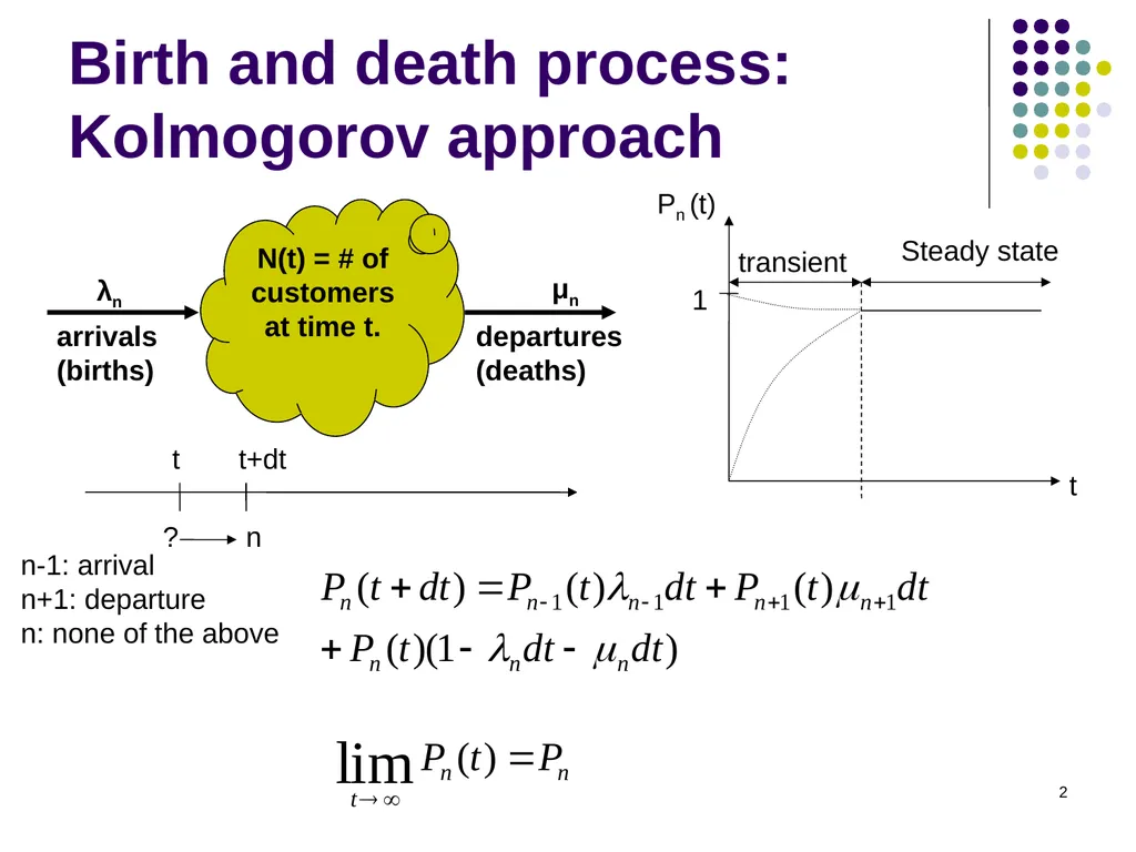
2 Birth and death process: Kolmogorov approach N(t) = # of customers
at time t. λn arrivals
(births) departures
(deaths) μn<br>
03
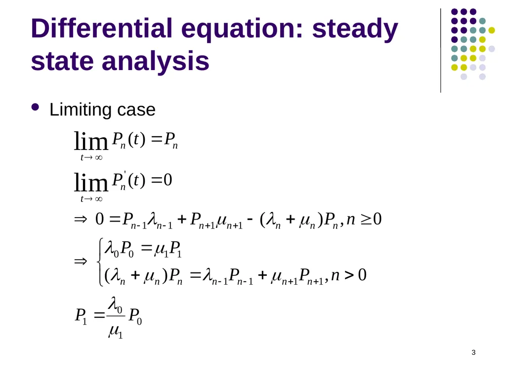
3 Differential equation: steady state analysis Limiting case<br>
04
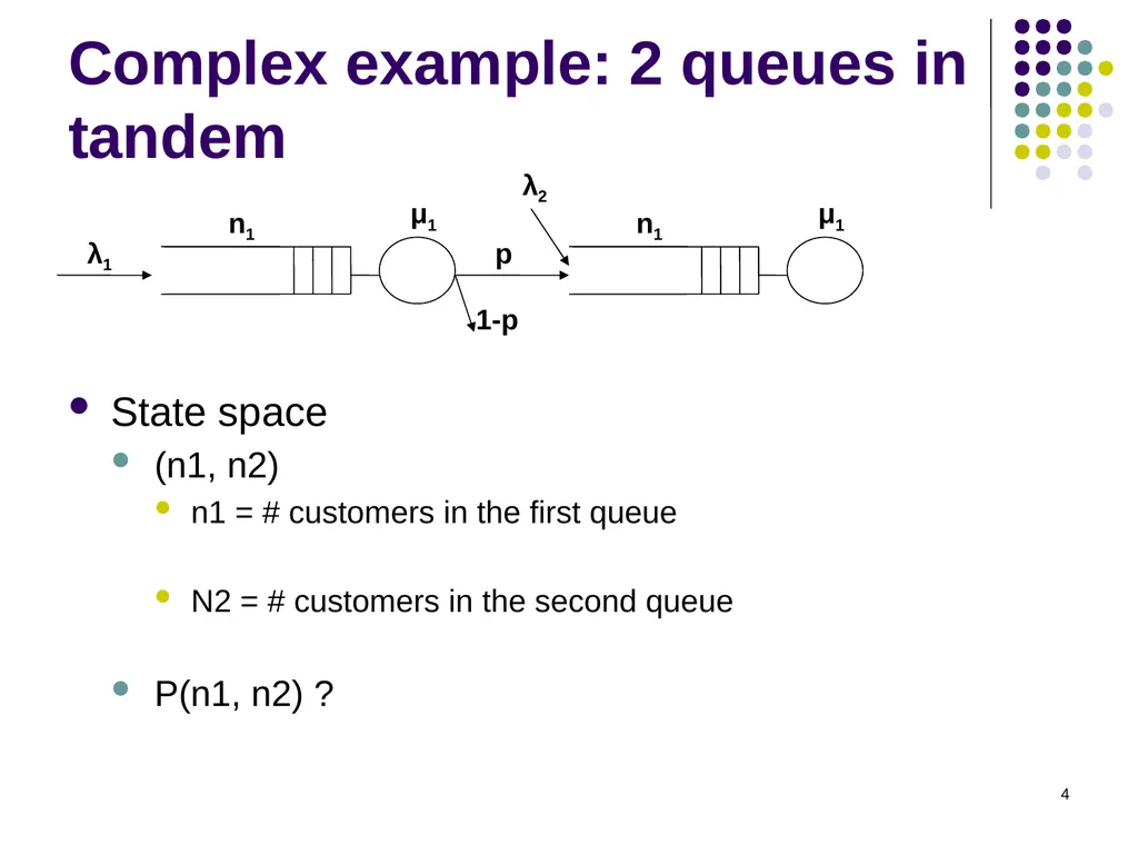
4 Complex example: 2 queues in tandem State space
(n1, n2)
n1 = # customers in the first queue
N2 = # customers in the second queue
P(n1, n2) ? λ1 μ1 n1 λ2 μ1 n1 p 1-p<br>
05
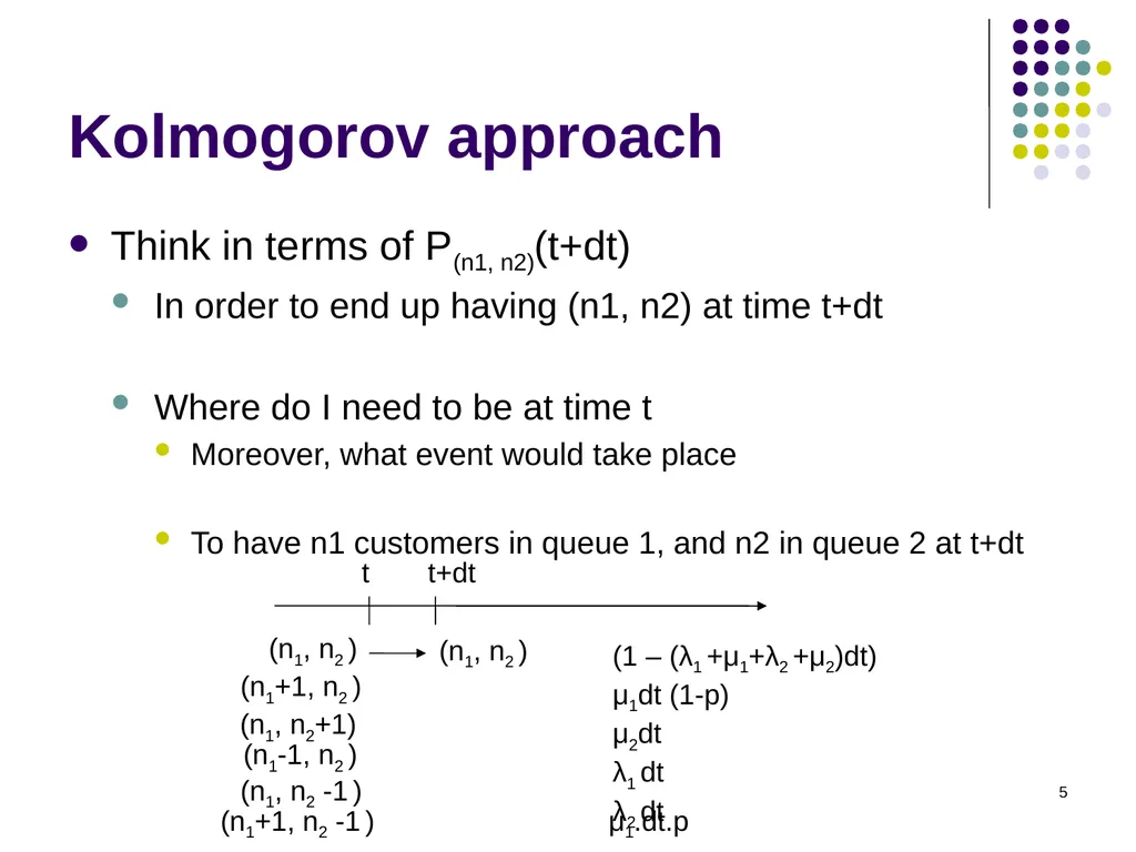
5 Kolmogorov approach Think in terms of P(n1, n2)(t+dt)
In order to end up having (n1, n2) at time t+dt
Where do I need to be at time t
Moreover, what event would take place
To have n1 customers in queue 1, and n2 in queue 2 at t+dt t+dt t (n1, n2 ) (n1, n2 ) (n1+1, n2 ) (n1, n2+1) (n1-1, n2 ) (n1, n2 -1 ) (1 – (λ1 +μ1+λ2 +μ2)dt)
μ1dt (1-p)
μ2dt
λ1 dt
λ2 dt (n1+1, n2 -1 ) μ1.dt.p<br>
06
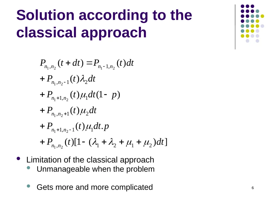
6 Solution according to the classical approach Limitation of the classical approach
Unmanageable when the problem
Gets more and more complicated<br>
07
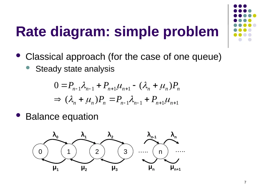
7 Rate diagram: simple problem Classical approach (for the case of one queue)
Steady state analysis
Balance equation 0 1 2 3 ….. n …..<br>
08
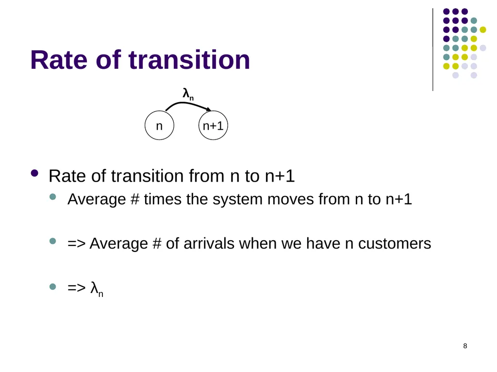
8 Rate of transition Rate of transition from n to n+1
Average # times the system moves from n to n+1
=> Average # of arrivals when we have n customers
=> λn n n+1<br>
09
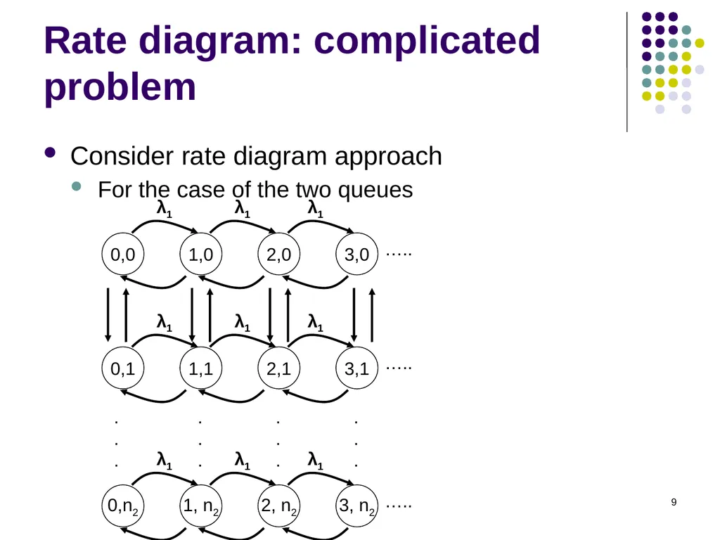
9 Rate diagram: complicated problem Consider rate diagram approach
For the case of the two queues .
.
. .
.
. .
.
. .
.
.<br>
10
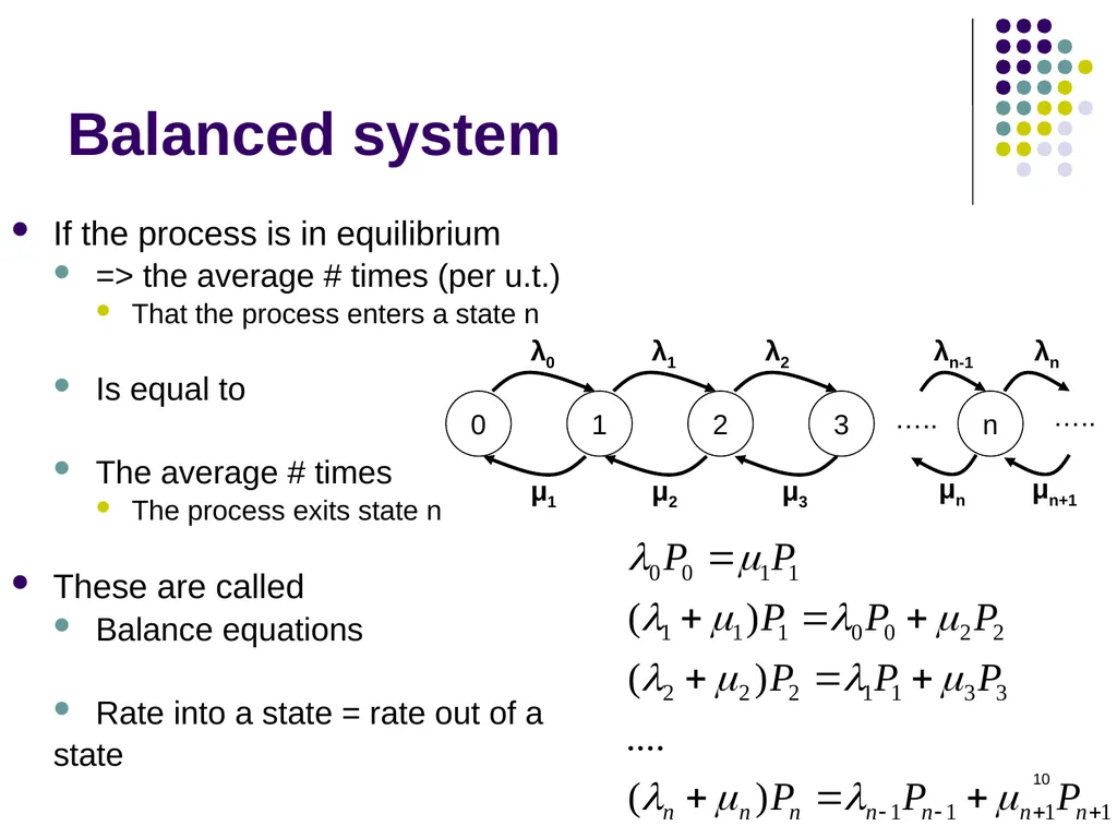
10 Balanced system If the process is in equilibrium
=> the average # times (per u.t.)
That the process enters a state n
Is equal to
The average # times
The process exits state n
These are called
Balance equations
Rate into a state = rate out of a
state<br>
11
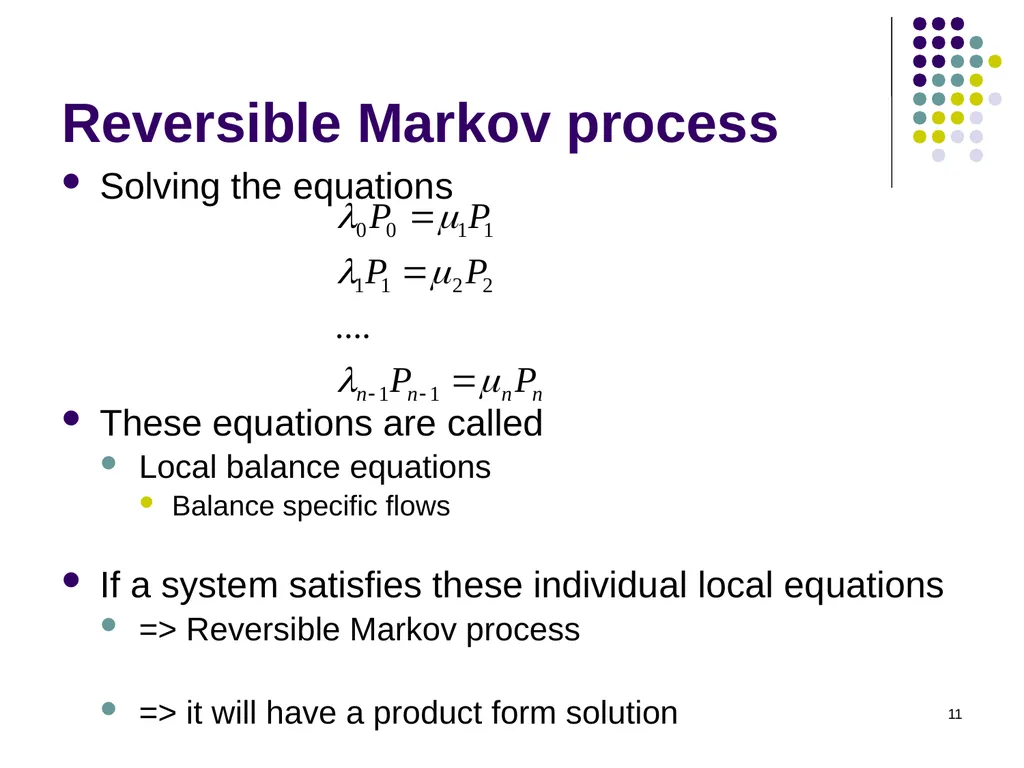
11 Reversible Markov process Solving the equations
These equations are called
Local balance equations
Balance specific flows
If a system satisfies these individual local equations
=> Reversible Markov process
=> it will have a product form solution<br>
12
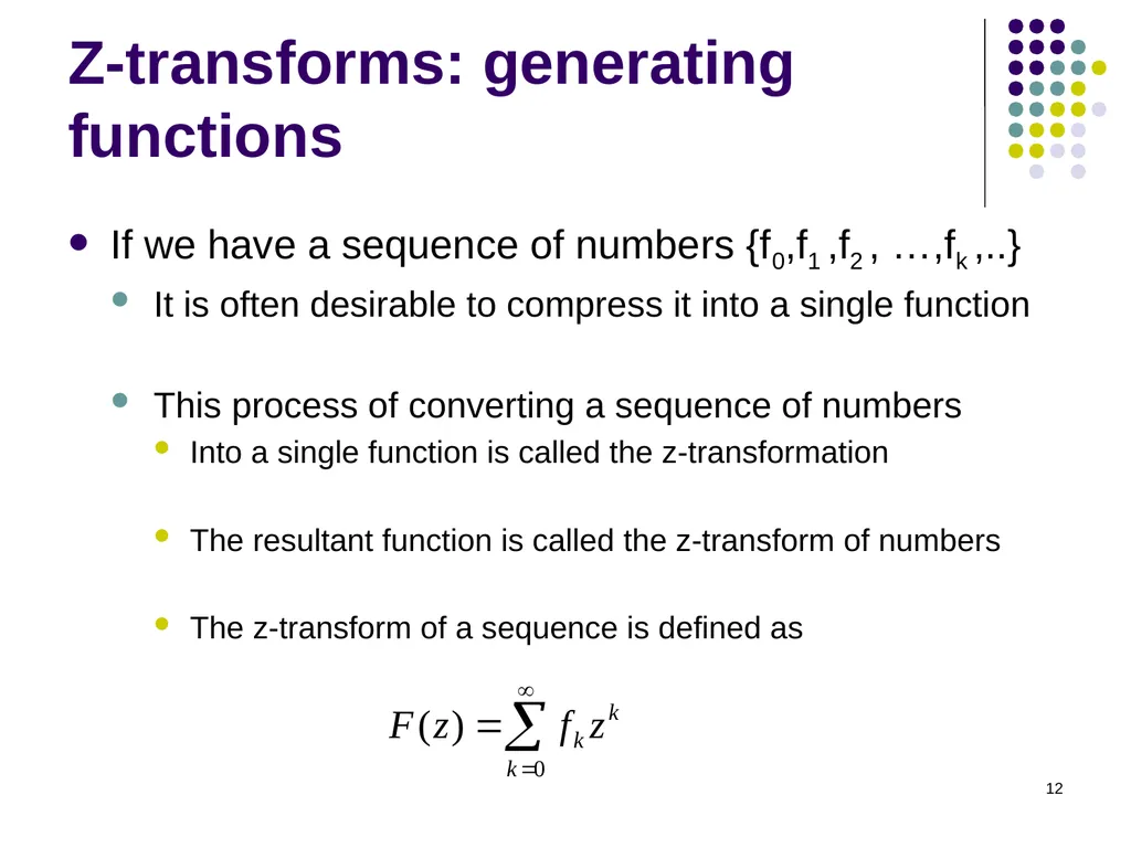
12 Z-transforms: generating functions If we have a sequence of numbers {f0,f1 ,f2 , …,fk ,..}
It is often desirable to compress it into a single function
This process of converting a sequence of numbers
Into a single function is called the z-transformation
The resultant function is called the z-transform of numbers
The z-transform of a sequence is defined as<br>
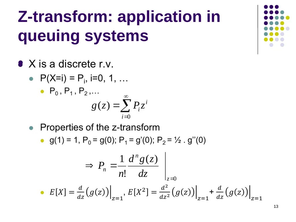
13
13 Z-transform: application in queuing systems<br>