
Chapter 10: Big Data Motivation Very large volumes
Description: Chapter 10: Big Data Motivation Very large volumes of data being collected Driven by growth of web, social media, and more recently internet-of-things Web logs were an early source of data Analytics on web logs has great value for
Related Topics
Download Presentation
"Chapter 10: Big Data Motivation Very large volumes" is the property of its rightful owner. Permission is granted to download and print the materials on this website for personal, non-commercial use only, and to display it on your personal computer provided you do not modify the materials and that you retain all copyright notices contained in the materials. By downloading content from our website, you accept the terms of this agreement.
Presentation Transcript
slide1. Chapter 10: Big Data<br>
slide2. Motivation Very large volumes of data being collected
Driven by growth of web, social media, and more recently internet-of-things
Web logs were an early source of data
Analytics on web logs has great value for advertisements, web site structuring, what posts to show to a user, etc
Big Data: differentiated from data handled by earlier generation databases
Volume: much larger amounts of data stored
Velocity: much higher rates of insertions
Variety: many types of data, beyond relational data<br>
slide3. Querying Big Data Transaction processing systems that need very high scalability
Many applications willing to sacrifice ACID properties and other database features, if they can get very high scalability
Query processing systems that
Need very high scalability, and
Need to support non-relation data<br>
slide4. Big Data Storage Systems Distributed file systems
Shardring across multiple databases
Key-value storage systems
Parallel and distributed databases<br>
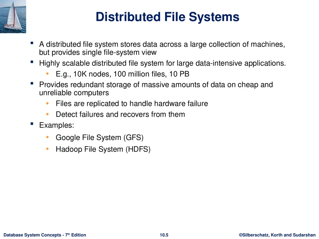
slide5. Distributed File Systems A distributed file system stores data across a large collection of machines, but provides single file-system view
Highly scalable distributed file system for large data-intensive applications.
E.g., 10K nodes, 100 million files, 10 PB
Provides redundant storage of massive amounts of data on cheap and unreliable computers
Files are replicated to handle hardware failure
Detect failures and recovers from them
Examples:
Google File System (GFS)
Hadoop File System (HDFS)<br>
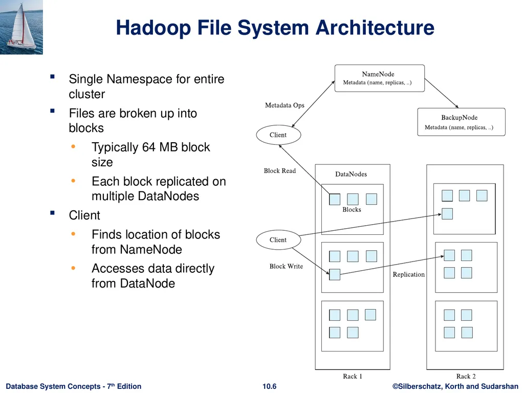
slide6. Hadoop File System Architecture Single Namespace for entire cluster
Files are broken up into blocks
Typically 64 MB block size
Each block replicated on multiple DataNodes
Client
Finds location of blocks from NameNode
Accesses data directly from DataNode<br>
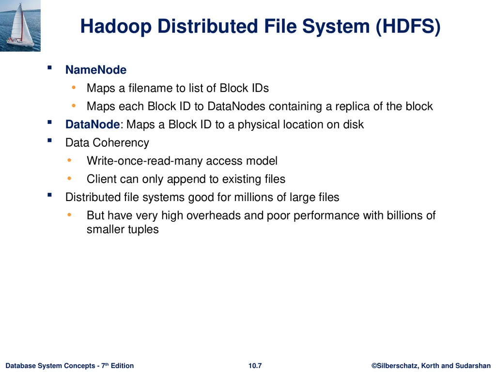
slide7. Hadoop Distributed File System (HDFS) NameNode
Maps a filename to list of Block IDs
Maps each Block ID to DataNodes containing a replica of the block
DataNode: Maps a Block ID to a physical location on disk
Data Coherency
Write-once-read-many access model
Client can only append to existing files
Distributed file systems good for millions of large files
But have very high overheads and poor performance with billions of smaller tuples<br>
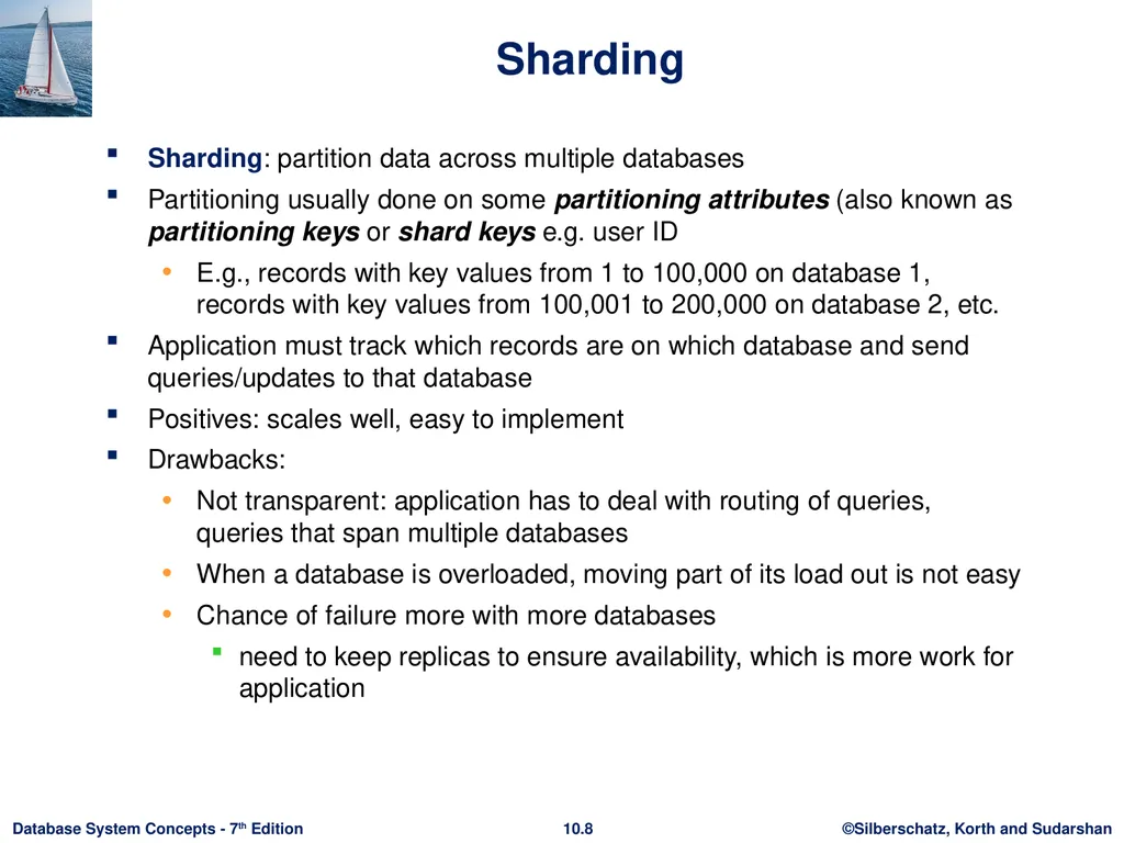
slide8. Sharding Sharding: partition data across multiple databases
Partitioning usually done on some partitioning attributes (also known as partitioning keys or shard keys e.g. user ID
E.g., records with key values from 1 to 100,000 on database 1, records with key values from 100,001 to 200,000 on database 2, etc.
Application must track which records are on which database and send queries/updates to that database
Positives: scales well, easy to implement
Drawbacks:
Not transparent: application has to deal with routing of queries, queries that span multiple databases
When a database is overloaded, moving part of its load out is not easy
Chance of failure more with more databases
need to keep replicas to ensure availability, which is more work for application<br>
slide9. Parallel Databases and Data Stores Supporting scalable data access
Approach 1: memcache or other caching mechanisms at application servers, to reduce database access
Limited in scalability
Approach 2: Partition (“shard”) data across multiple separate database servers
Approach 3: Use existing parallel databases
Historically: parallel databases that can scale to large number of machines were designed for decision support not OLTP
Approach 4: Massively Parallel Key-Value Data Store
Partitioning, high availability etc. completely transparent to application
Sharding systems and key-value stores don’t support many relational features, such as joins, integrity constraints, etc., across partitions.<br>
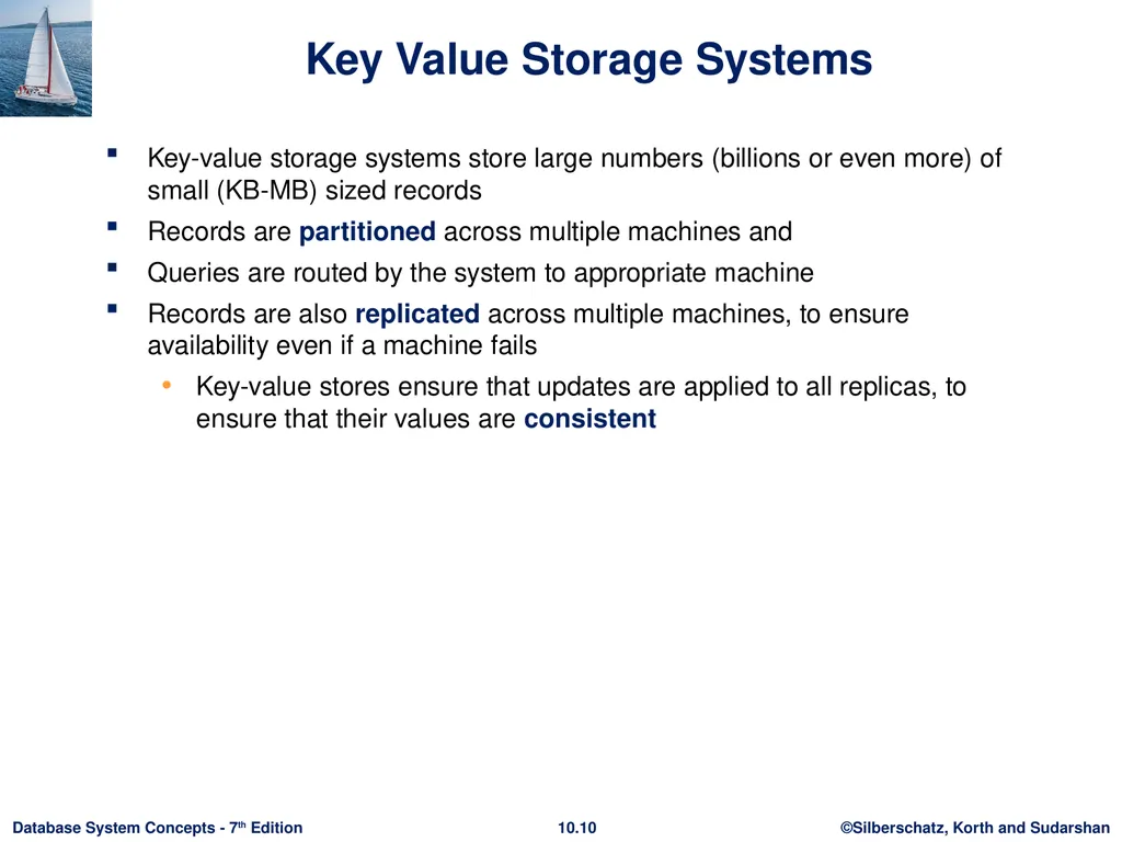
slide10. Key Value Storage Systems Key-value storage systems store large numbers (billions or even more) of small (KB-MB) sized records
Records are partitioned across multiple machines and
Queries are routed by the system to appropriate machine
Records are also replicated across multiple machines, to ensure availability even if a machine fails
Key-value stores ensure that updates are applied to all replicas, to ensure that their values are consistent<br>
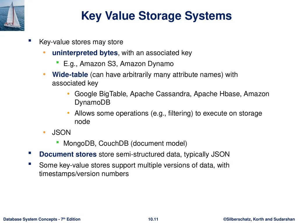
slide11. Key Value Storage Systems Key-value stores may store
uninterpreted bytes, with an associated key
E.g., Amazon S3, Amazon Dynamo
Wide-table (can have arbitrarily many attribute names) with associated key
Google BigTable, Apache Cassandra, Apache Hbase, Amazon DynamoDB
Allows some operations (e.g., filtering) to execute on storage node
JSON
MongoDB, CouchDB (document model)
Document stores store semi-structured data, typically JSON
Some key-value stores support multiple versions of data, with timestamps/version numbers<br>
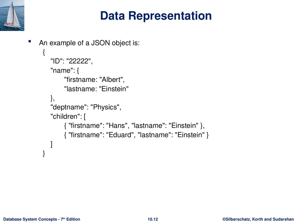
slide12. Data Representation An example of a JSON object is:
{
"ID": "22222",
"name": {
"firstname: "Albert",
"lastname: "Einstein"
},
"deptname": "Physics",
"children": [
{ "firstname": "Hans", "lastname": "Einstein" },
{ "firstname": "Eduard", "lastname": "Einstein" }
]
}<br>
slide13. Key Value Storage Systems Key-value stores support
put(key, value): used to store values with an associated key,
get(key): which retrieves the stored value associated with the specified key
delete(key) -- Remove the key and its associated value
Some systems also support range queries on key values
Document stores also support queries on non-key attributes
See book for MongoDB queries
Key value stores are not full database systems
Have no/limited support for transactional updates
Applications must manage query processing on their own
Not supporting above features makes it easier to build scalable data storage systems
Also called NoSQL systems<br>
slide14. Parallel and Distributed Databases Parallel databases run multiple machines (cluser)
Developed in 1980s, well before Big Data
Parallel databases were designed for smaller scale (10s to 100s of machines)
Did not provide easy scalability
Replication used to ensure data availability despite machine failure
But typically restart query in event of failure
Restarts may be frequent at very large scale
Map-reduce systems (coming up next) can continue query execution, working around failures<br>
slide15. Replication and Consistency Availability (system can run even if parts have failed) is essential for parallel/distributed databases
Via replication, so even if a node has failed, another copy is available
Consistency is important for replicated data
All live replicas have same value, and each read sees latest version
Often implemented using majority protocols
E.g., have 3 replicas, reads/writes must access 2 replicas
Details in chapter 23
Network partitions (network can break into two or more parts, each with active systems that can’t talk to other parts)
In presence of partitions, cannot guarantee both availability and consistency
Brewer’s CAP “Theorem”<br>
slide16. Replication and Consistency Very large systems will partition at some point
Choose one of consistency or availability
Traditional database choose consistency
Most Web applications choose availability
Except for specific parts such as order processing
More details later, in Chapter 23<br>
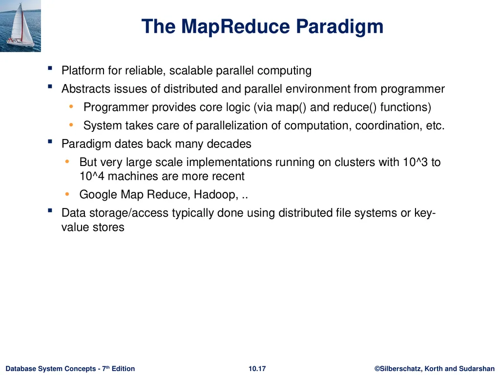
slide17. The MapReduce Paradigm Platform for reliable, scalable parallel computing
Abstracts issues of distributed and parallel environment from programmer
Programmer provides core logic (via map() and reduce() functions)
System takes care of parallelization of computation, coordination, etc.
Paradigm dates back many decades
But very large scale implementations running on clusters with 10^3 to 10^4 machines are more recent
Google Map Reduce, Hadoop, ..
Data storage/access typically done using distributed file systems or key-value stores<br>
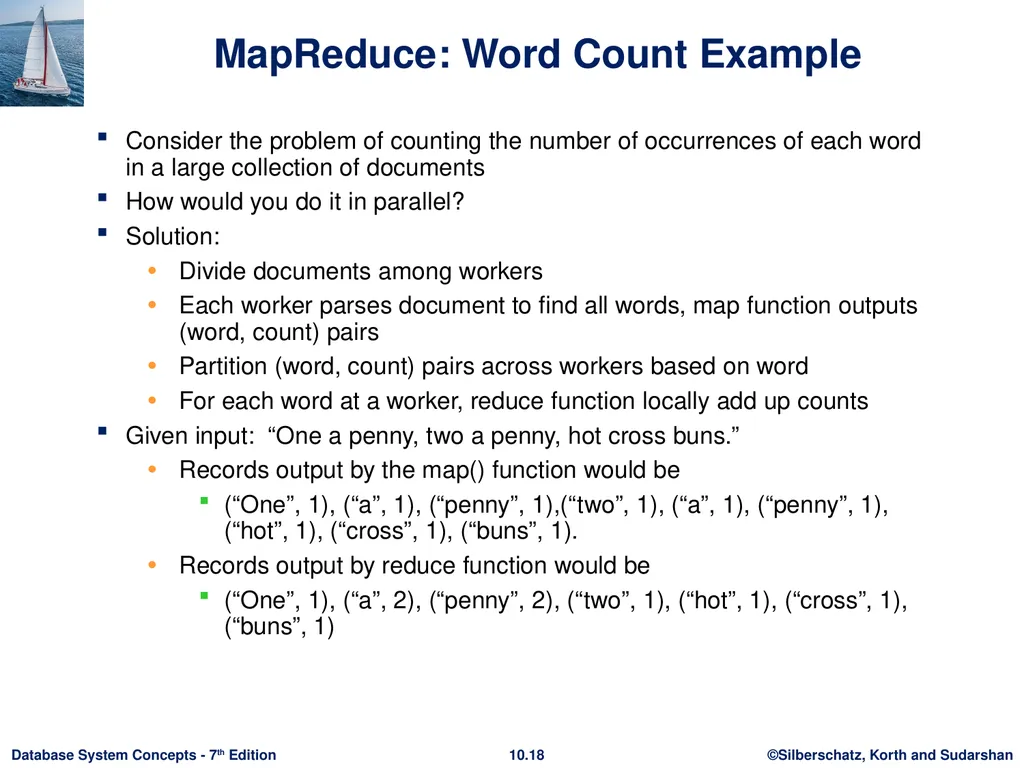
slide18. MapReduce: Word Count Example Consider the problem of counting the number of occurrences of each word in a large collection of documents
How would you do it in parallel?
Solution:
Divide documents among workers
Each worker parses document to find all words, map function outputs (word, count) pairs
Partition (word, count) pairs across workers based on word
For each word at a worker, reduce function locally add up counts
Given input: “One a penny, two a penny, hot cross buns.”
Records output by the map() function would be
(“One”, 1), (“a”, 1), (“penny”, 1),(“two”, 1), (“a”, 1), (“penny”, 1), (“hot”, 1), (“cross”, 1), (“buns”, 1).
Records output by reduce function would be
(“One”, 1), (“a”, 2), (“penny”, 2), (“two”, 1), (“hot”, 1), (“cross”, 1), (“buns”, 1)<br>
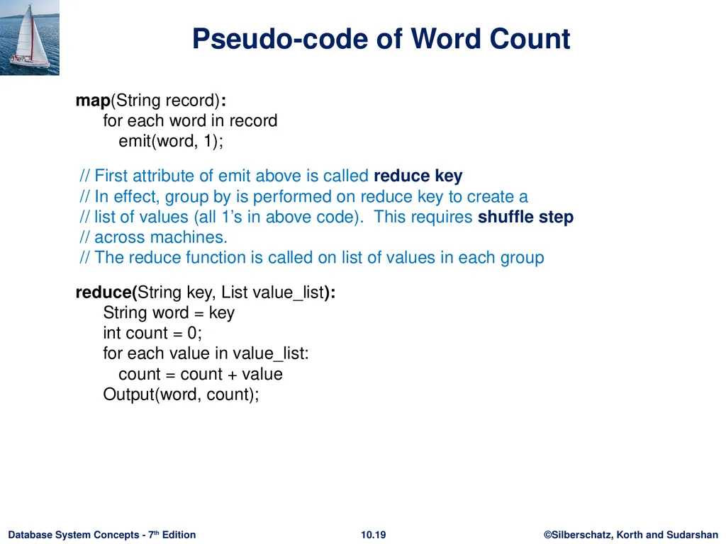
slide19. Pseudo-code of Word Count map(String record):
for each word in record
emit(word, 1);
// First attribute of emit above is called reduce key
// In effect, group by is performed on reduce key to create a
// list of values (all 1’s in above code). This requires shuffle step
// across machines.
// The reduce function is called on list of values in each group
reduce(String key, List value_list):
String word = key
int count = 0;
for each value in value_list:
count = count + value
Output(word, count);<br>
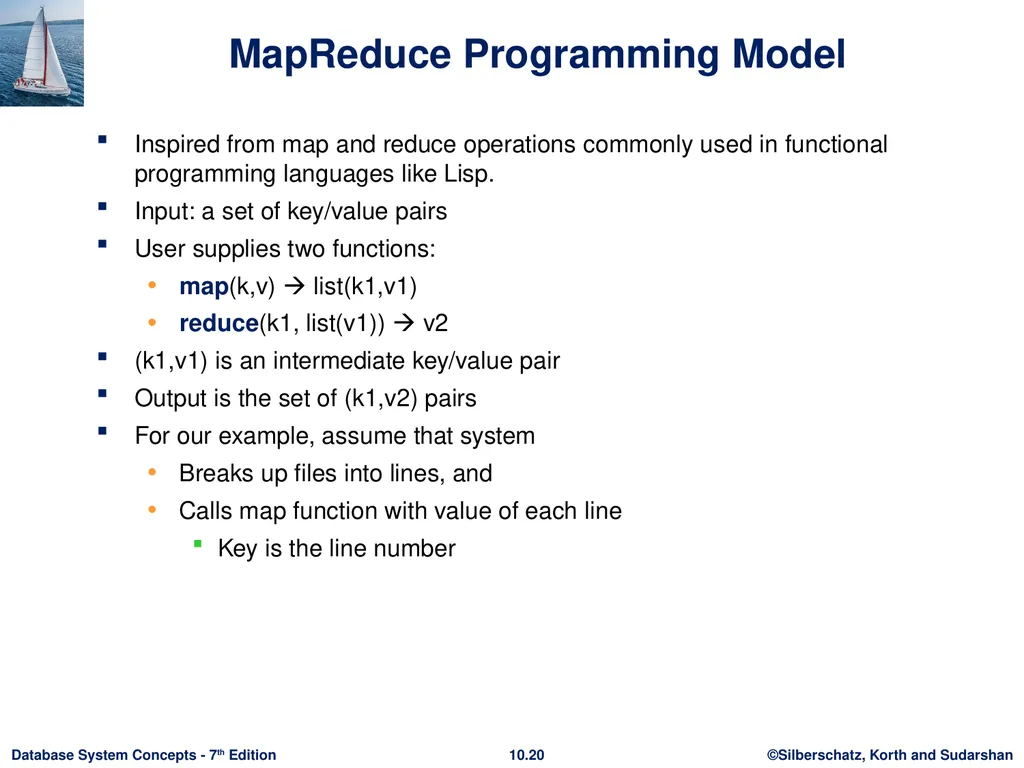
slide20. MapReduce Programming Model Inspired from map and reduce operations commonly used in functional programming languages like Lisp.
Input: a set of key/value pairs
User supplies two functions:
map(k,v) list(k1,v1)
reduce(k1, list(v1)) v2
(k1,v1) is an intermediate key/value pair
Output is the set of (k1,v2) pairs
For our example, assume that system
Breaks up files into lines, and
Calls map function with value of each line
Key is the line number<br>
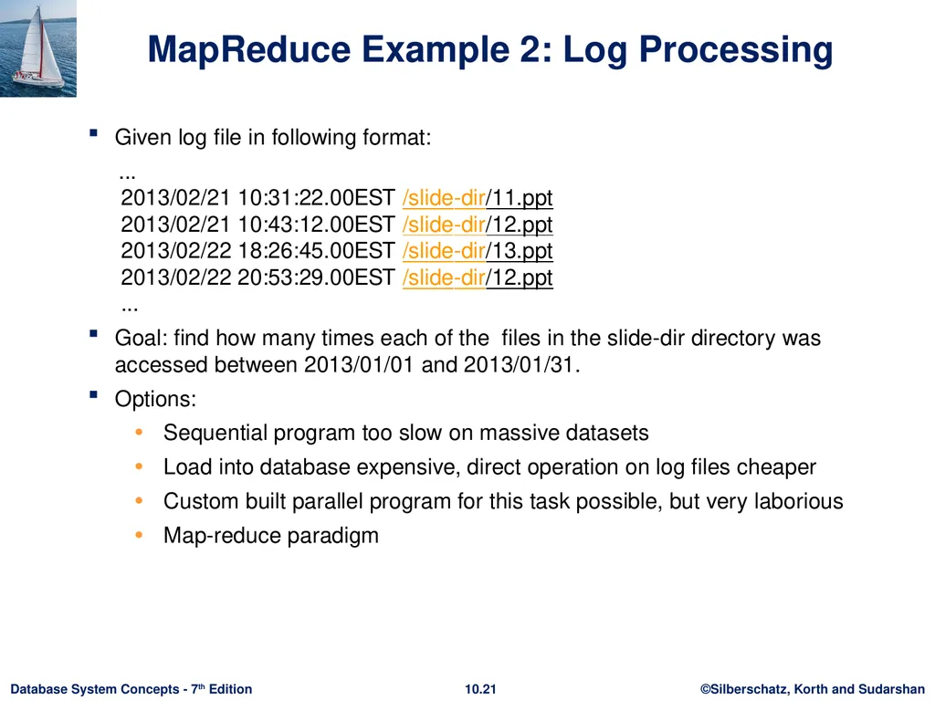
slide21. MapReduce Example 2: Log Processing Given log file in following format:
... 2013/02/21 10:31:22.00EST /slide-dir/11.ppt 2013/02/21 10:43:12.00EST /slide-dir/12.ppt 2013/02/22 18:26:45.00EST /slide-dir/13.ppt 2013/02/22 20:53:29.00EST /slide-dir/12.ppt ...
Goal: find how many times each of the files in the slide-dir directory was accessed between 2013/01/01 and 2013/01/31.
Options:
Sequential program too slow on massive datasets
Load into database expensive, direct operation on log files cheaper
Custom built parallel program for this task possible, but very laborious
Map-reduce paradigm<br>
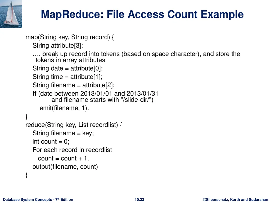
slide22. MapReduce: File Access Count Example map(String key, String record) {
String attribute[3];
…. break up record into tokens (based on space character), and store the tokens in array attributes
String date = attribute[0];
String time = attribute[1];
String filename = attribute[2];
if (date between 2013/01/01 and 2013/01/31 and filename starts with "/slide-dir/")
emit(filename, 1).
}
reduce(String key, List recordlist) {
String filename = key;
int count = 0;
For each record in recordlist
count = count + 1.
output(filename, count)
}<br>
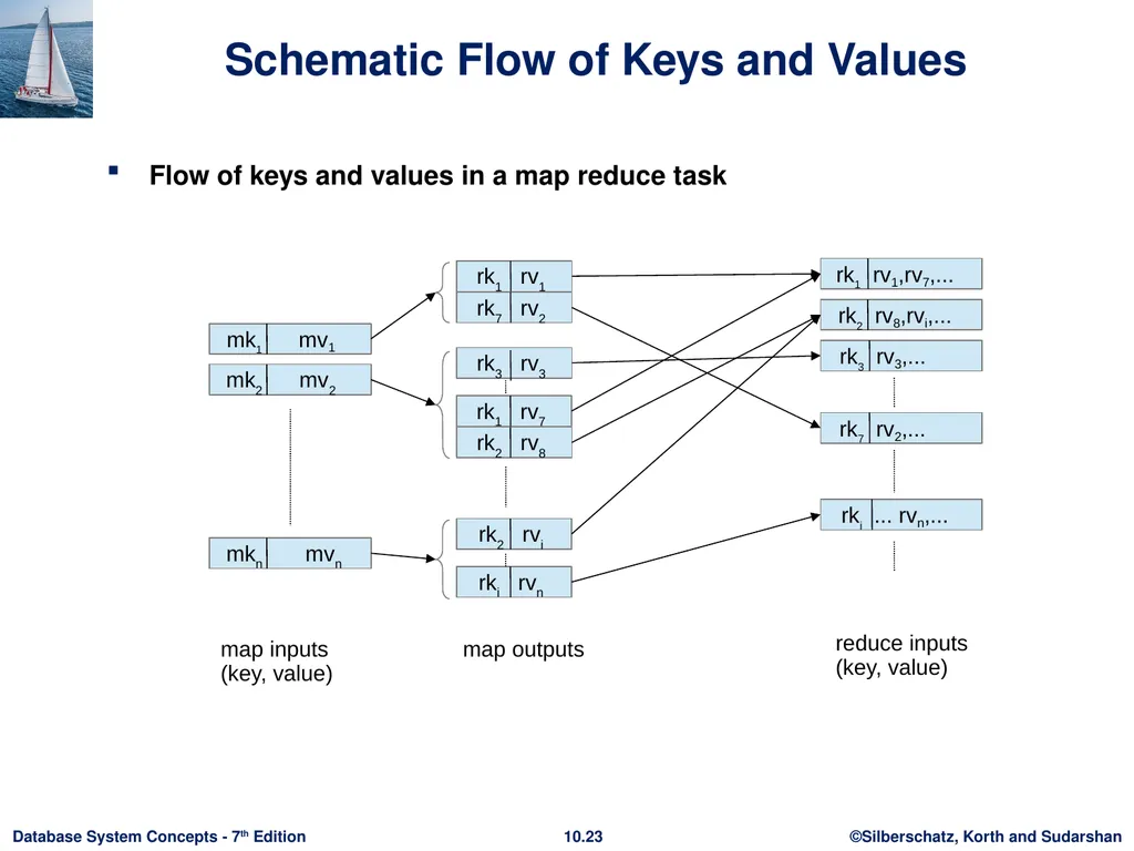
slide23. Schematic Flow of Keys and Values Flow of keys and values in a map reduce task<br>
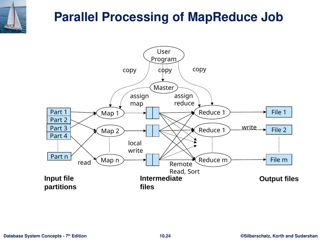
slide24. Parallel Processing of MapReduce Job<br>
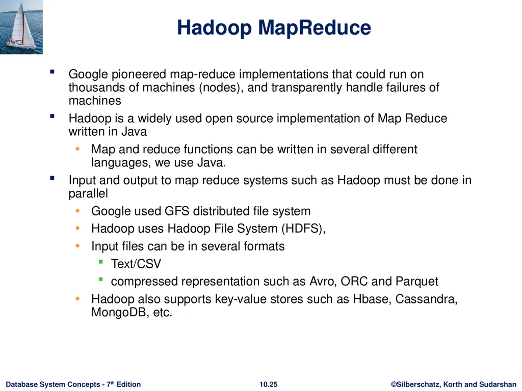
slide25. Hadoop MapReduce Google pioneered map-reduce implementations that could run on thousands of machines (nodes), and transparently handle failures of machines
Hadoop is a widely used open source implementation of Map Reduce written in Java
Map and reduce functions can be written in several different languages, we use Java.
Input and output to map reduce systems such as Hadoop must be done in parallel
Google used GFS distributed file system
Hadoop uses Hadoop File System (HDFS),
Input files can be in several formats
Text/CSV
compressed representation such as Avro, ORC and Parquet
Hadoop also supports key-value stores such as Hbase, Cassandra, MongoDB, etc.<br>
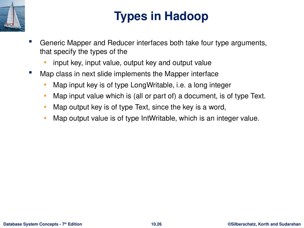
slide26. Types in Hadoop Generic Mapper and Reducer interfaces both take four type arguments, that specify the types of the
input key, input value, output key and output value
Map class in next slide implements the Mapper interface
Map input key is of type LongWritable, i.e. a long integer
Map input value which is (all or part of) a document, is of type Text.
Map output key is of type Text, since the key is a word,
Map output value is of type IntWritable, which is an integer value.<br>
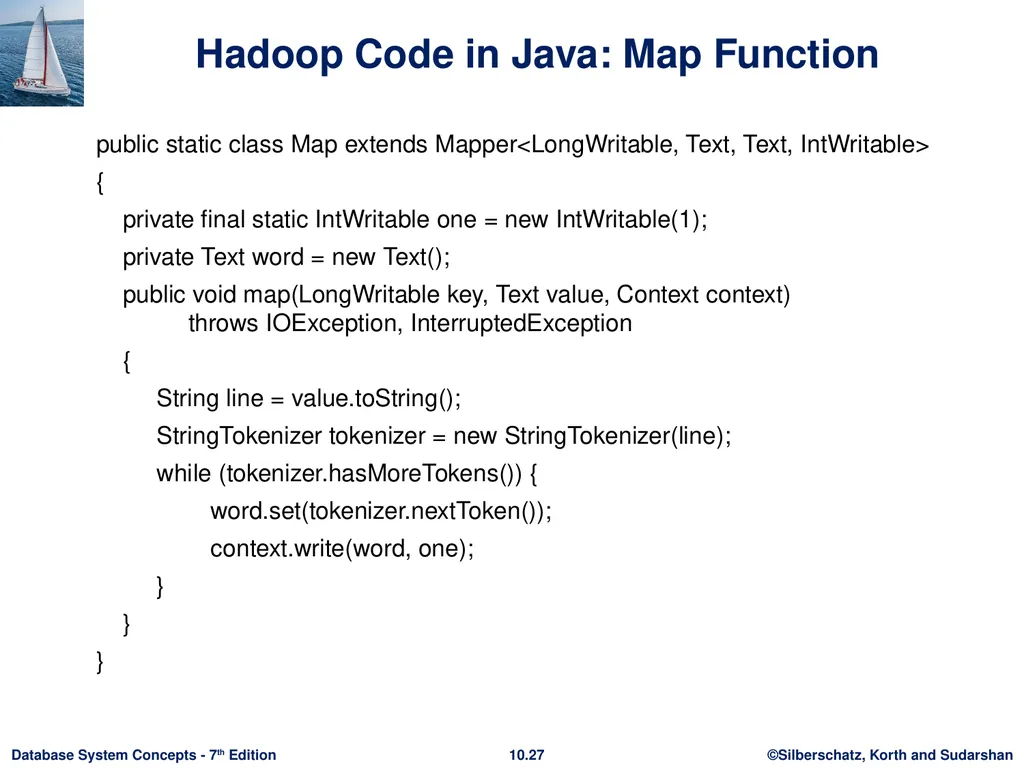
slide27. Hadoop Code in Java: Map Function public static class Map extends Mapper<LongWritable, Text, Text, IntWritable>
{
private final static IntWritable one = new IntWritable(1);
private Text word = new Text();
public void map(LongWritable key, Text value, Context context) throws IOException, InterruptedException
{
String line = value.toString();
StringTokenizer tokenizer = new StringTokenizer(line);
while (tokenizer.hasMoreTokens()) {
word.set(tokenizer.nextToken());
context.write(word, one);
}
}
}<br>
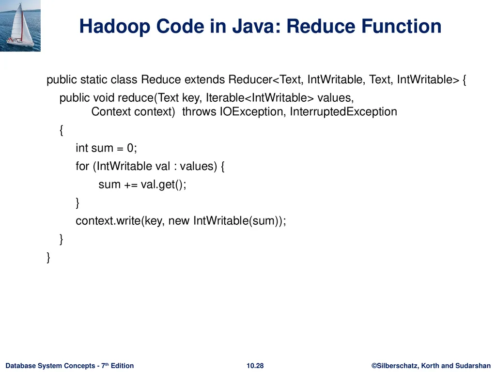
slide28. Hadoop Code in Java: Reduce Function public static class Reduce extends Reducer<Text, IntWritable, Text, IntWritable> {
public void reduce(Text key, Iterable<IntWritable> values, Context context) throws IOException, InterruptedException
{
int sum = 0;
for (IntWritable val : values) {
sum += val.get();
}
context.write(key, new IntWritable(sum));
}
}<br>
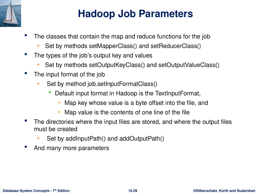
slide29. Hadoop Job Parameters The classes that contain the map and reduce functions for the job
Set by methods setMapperClass() and setReducerClass()
The types of the job’s output key and values
Set by methods setOutputKeyClass() and setOutputValueClass()
The input format of the job
Set by method job.setInputFormatClass()
Default input format in Hadoop is the TextInputFormat,
Map key whose value is a byte offset into the file, and
Map value is the contents of one line of the file
The directories where the input files are stored, and where the output files must be created
Set by addInputPath() and addOutputPath()
And many more parameters<br>
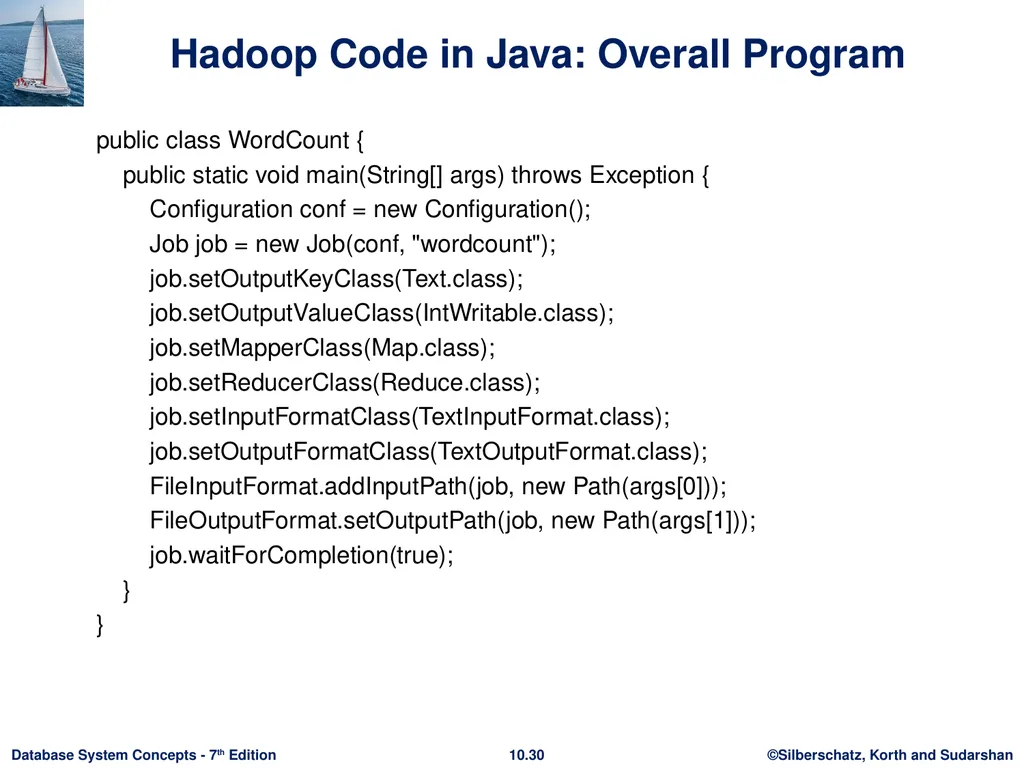
slide30. Hadoop Code in Java: Overall Program public class WordCount {
public static void main(String[] args) throws Exception {
Configuration conf = new Configuration();
Job job = new Job(conf, "wordcount");
job.setOutputKeyClass(Text.class);
job.setOutputValueClass(IntWritable.class);
job.setMapperClass(Map.class);
job.setReducerClass(Reduce.class);
job.setInputFormatClass(TextInputFormat.class);
job.setOutputFormatClass(TextOutputFormat.class);
FileInputFormat.addInputPath(job, new Path(args[0]));
FileOutputFormat.setOutputPath(job, new Path(args[1]));
job.waitForCompletion(true);
}
}<br>
slide31. Local Pre-Aggregation Combiners: perform partial aggregation to minimize network traffic
E.g., within machine
And/or at rack level
In Hadoop, reduce function is used by default if combiners are enabled
But alternative implementation of combiner can be specified if input and output types of reducers are different<br>
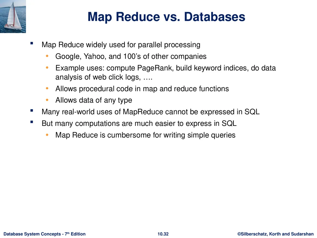
slide32. Map Reduce vs. Databases Map Reduce widely used for parallel processing
Google, Yahoo, and 100’s of other companies
Example uses: compute PageRank, build keyword indices, do data analysis of web click logs, ….
Allows procedural code in map and reduce functions
Allows data of any type
Many real-world uses of MapReduce cannot be expressed in SQL
But many computations are much easier to express in SQL
Map Reduce is cumbersome for writing simple queries<br>
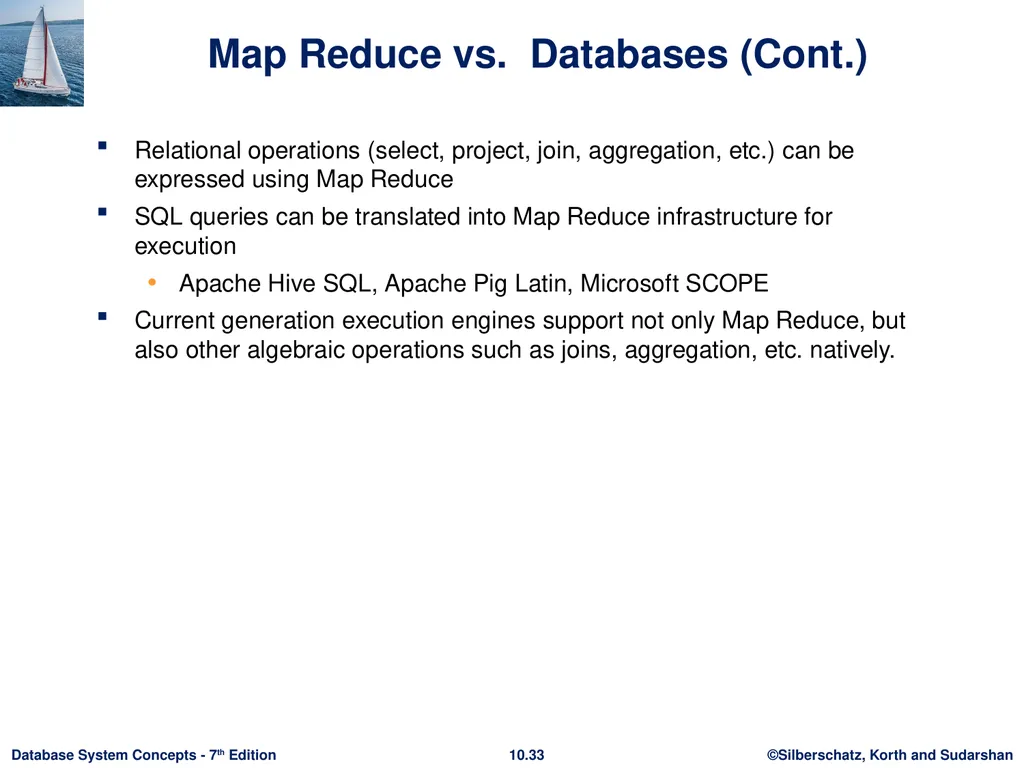
slide33. Map Reduce vs. Databases (Cont.) Relational operations (select, project, join, aggregation, etc.) can be expressed using Map Reduce
SQL queries can be translated into Map Reduce infrastructure for execution
Apache Hive SQL, Apache Pig Latin, Microsoft SCOPE
Current generation execution engines support not only Map Reduce, but also other algebraic operations such as joins, aggregation, etc. natively.<br>
slide34. Beyond MapReduce: Algebraic Operations<br>
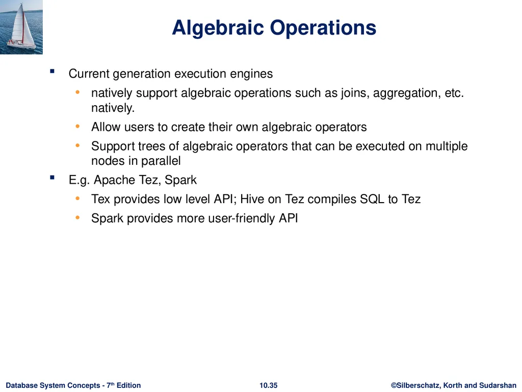
slide35. Algebraic Operations Current generation execution engines
natively support algebraic operations such as joins, aggregation, etc. natively.
Allow users to create their own algebraic operators
Support trees of algebraic operators that can be executed on multiple nodes in parallel
E.g. Apache Tez, Spark
Tex provides low level API; Hive on Tez compiles SQL to Tez
Spark provides more user-friendly API<br>
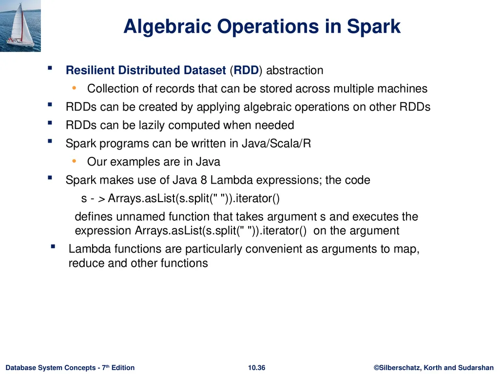
slide36. Algebraic Operations in Spark Resilient Distributed Dataset (RDD) abstraction
Collection of records that can be stored across multiple machines
RDDs can be created by applying algebraic operations on other RDDs
RDDs can be lazily computed when needed
Spark programs can be written in Java/Scala/R
Our examples are in Java
Spark makes use of Java 8 Lambda expressions; the code
s - > Arrays.asList(s.split(" ")).iterator()
defines unnamed function that takes argument s and executes the expression Arrays.asList(s.split(" ")).iterator() on the argument
Lambda functions are particularly convenient as arguments to map, reduce and other functions<br>
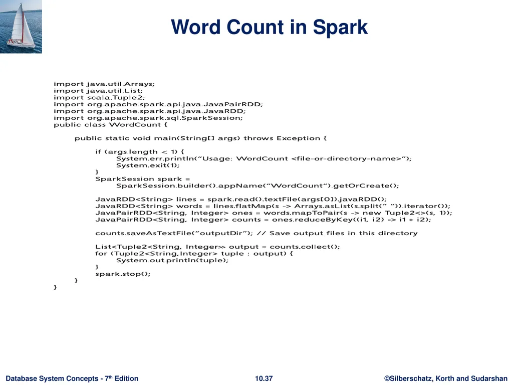
slide37. Word Count in Spark<br>
slide38. Algebraic Operations in Spark Algebraic operations in Spark are typically executed in parallel on multiple machines
With data partitioned across the machines
Algebraic operations are executed lazily, not immediately
Our preceding program creates an operator tree
Tree is executed only on specific functions such as saveAsTextFile() or collect()
Query optimization can be performed on tree before it is executed<br>
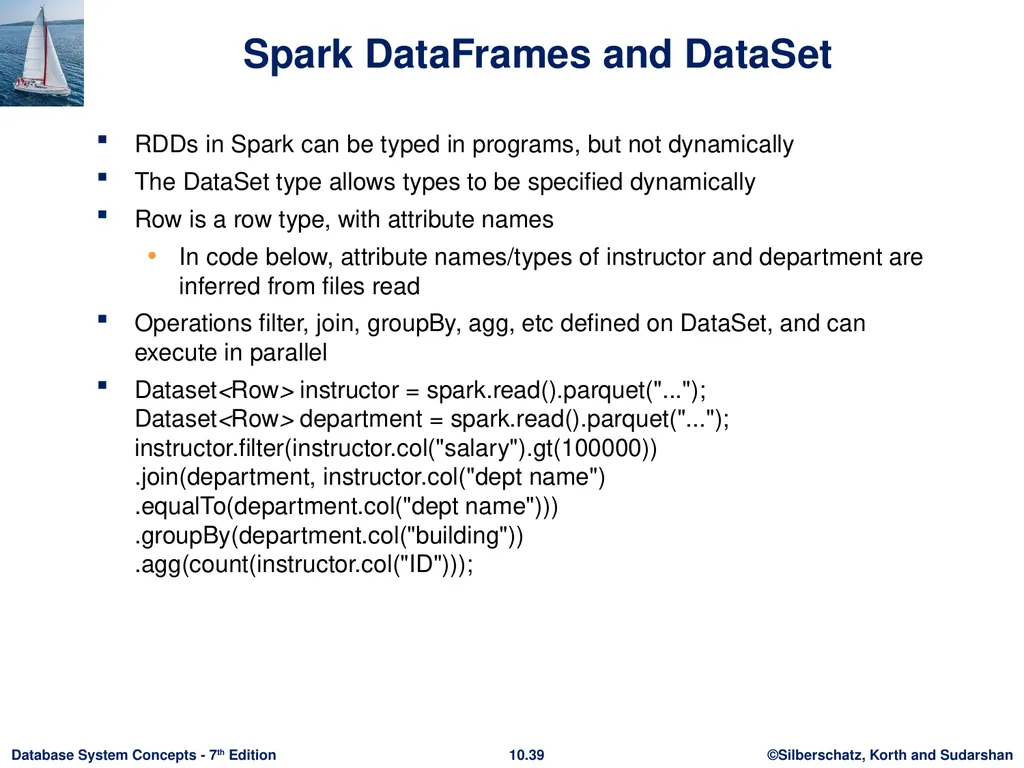
slide39. Spark DataFrames and DataSet RDDs in Spark can be typed in programs, but not dynamically
The DataSet type allows types to be specified dynamically
Row is a row type, with attribute names
In code below, attribute names/types of instructor and department are inferred from files read
Operations filter, join, groupBy, agg, etc defined on DataSet, and can execute in parallel
Dataset<Row> instructor = spark.read().parquet("..."); Dataset<Row> department = spark.read().parquet("..."); instructor.filter(instructor.col("salary").gt(100000)) .join(department, instructor.col("dept name") .equalTo(department.col("dept name"))) .groupBy(department.col("building")) .agg(count(instructor.col("ID")));<br>
slide40. Streaming Data<br>
slide41. Streaming Data and Applications Streaming data refers to data that arrives in a continuous fashion
Contrast to data-at-rest
Applications include:
Stock market: stream of trades
e-commerce site: purchases, searches
Sensors: sensor readings
Internet of things
Network monitoring data
Social media: tweets and posts can be viewed as a stream
Queries on streams can be very useful
Monitoring, alerts, automated triggering of actions<br>
slide42. Querying Streaming Data Windowing: Break up stream into windows, and queries are run on windows
Stream query languages support window operations
Windows may be based on time or tuples
Must figure out when all tuples in a window have been seen
Easy if stream totally ordered by timestamp
Punctuations specify that all future tuples have timestamp greater that some value
Continuous Queries: Queries written e.g. in SQL, output partial results based on stream seen so far; query results updated continuously
Have some applications, but can lead to flood of updates Approaches to querying streams:<br>
slide43. Querying Streaming Data (Cont.) Algebraic operators on streams:
Each operator consumes tuples from a stream and outputs tuples
Operators can be written e.g., in an imperative language
Operator may maintain state
Pattern matching:
Queries specify patterns, system detects occurrences of patterns and triggers actions
Complex Event Processing (CEP) systems
E.g., Microsoft StreamInsight, Flink CEP, Oracle Event Processing Approaches to querying streams (Cont.):<br>
slide44. Stream Processing Architectures Many stream processing systems are purely in-memory, and do not persist data
Lambda architecture: split stream into two, one output goes to stream processing system and the other to a database for storage
Easy to implement and widely used
But often leads to duplication of querying effort, once on streaming system and once in database<br>
slide45. Stream Extensions to SQL SQL Window functions described in Section 5.5.2
Streaming systems often support more window types
Tumbling window
E.g., hourly windows, windows don’t overlab
Hopping window
E.g., hourly window computed every 20 minutes
Sliding window
Window of specified size (based on timestamp interval or number of tuples) around each incoming tuple
Session window
Groups tuples based on user sessions<br>
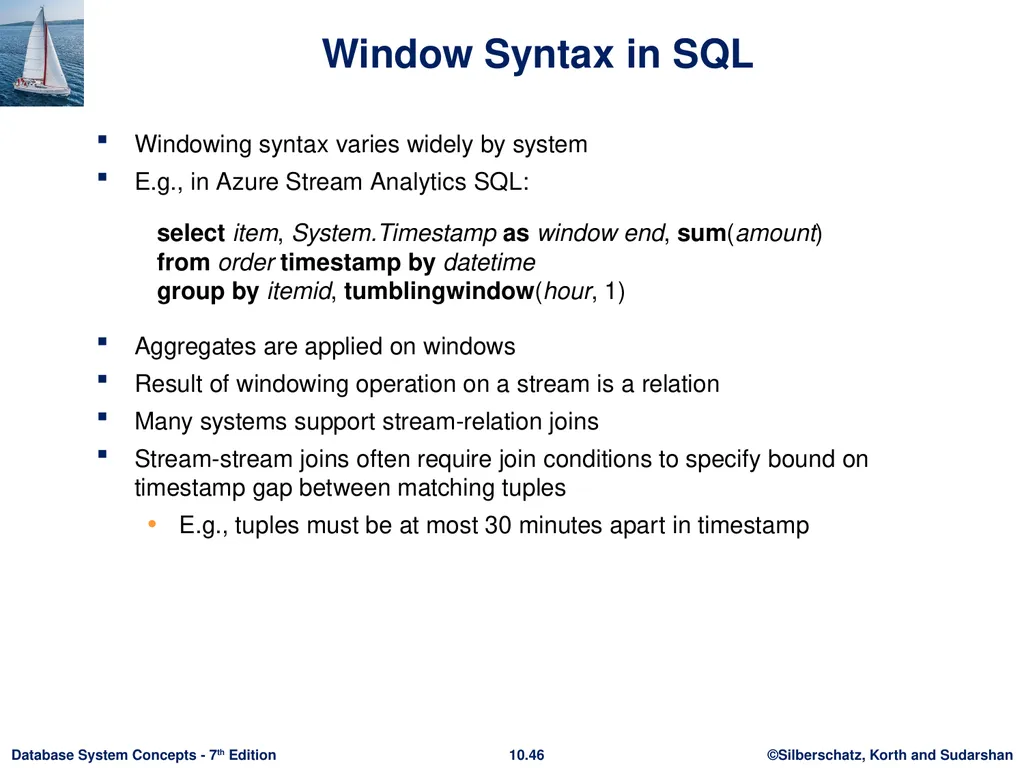
slide46. Window Syntax in SQL Windowing syntax varies widely by system
E.g., in Azure Stream Analytics SQL:
select item, System.Timestamp as window end, sum(amount) from order timestamp by datetime group by itemid, tumblingwindow(hour, 1)
Aggregates are applied on windows
Result of windowing operation on a stream is a relation
Many systems support stream-relation joins
Stream-stream joins often require join conditions to specify bound on timestamp gap between matching tuples
E.g., tuples must be at most 30 minutes apart in timestamp<br>
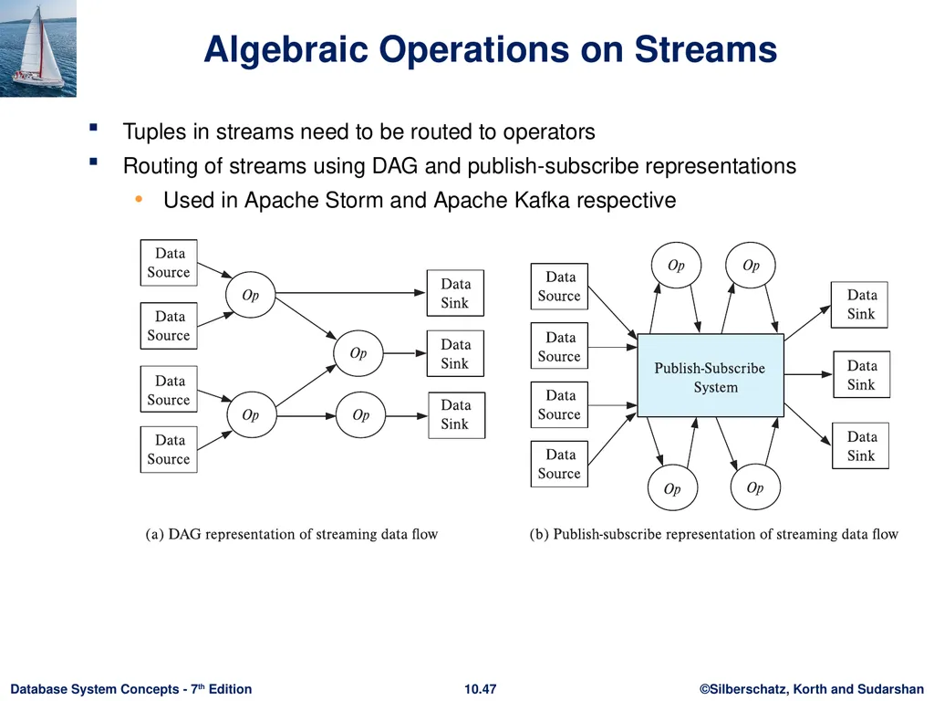
slide47. Algebraic Operations on Streams Tuples in streams need to be routed to operators
Routing of streams using DAG and publish-subscribe representations
Used in Apache Storm and Apache Kafka respective<br>
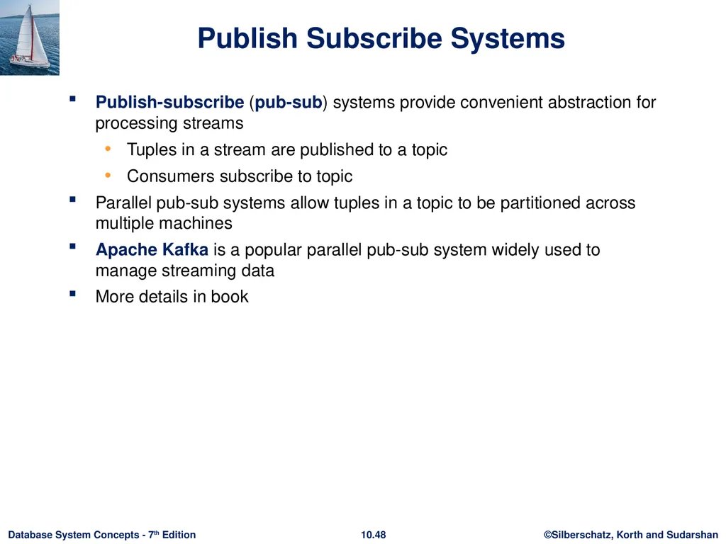
slide48. Publish Subscribe Systems Publish-subscribe (pub-sub) systems provide convenient abstraction for processing streams
Tuples in a stream are published to a topic
Consumers subscribe to topic
Parallel pub-sub systems allow tuples in a topic to be partitioned across multiple machines
Apache Kafka is a popular parallel pub-sub system widely used to manage streaming data
More details in book<br>
slide49. Graph Databases<br>
slide50. Graph Data Model Graphs are a very general data model
ER model of an enterprise can be viewed as a graph
Every entity is a node
Every binary relationship is an edge
Ternary and higher degree relationships can be modelled as binary relationships<br>
slide51. Graph Data Model (Cont.) Graphs can be modelled as relations
node(ID, label, node_data)
edge(fromID, toID, label, edge_data)
Above representation too simplistic
Graph databases like Neo4J can provide a graph view of relational schema
Relations can be identified as representing either nodes or edges
Query languages for graph databases make it
easy to express queries requiring edge traversal
allow efficient algorithms to be used for evaluation<br>
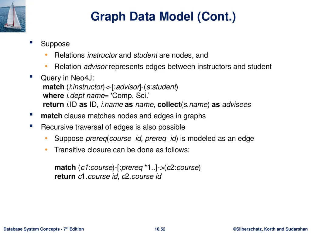
slide52. Graph Data Model (Cont.) Suppose
Relations instructor and student are nodes, and
Relation advisor represents edges between instructors and student
Query in Neo4J: match (i:instructor)<-[:advisor]-(s:student) where i.dept name= 'Comp. Sci.’ return i.ID as ID, i.name as name, collect(s.name) as advisees
match clause matches nodes and edges in graphs
Recursive traversal of edges is also possible
Suppose prereq(course_id, prereq_id) is modeled as an edge
Transitive closure can be done as follows: match (c1:course)-[:prereq *1..]->(c2:course) return c1.course id, c2.course id<br>
slide53. Parallel Graph Processing Very large graphs (billions of nodes, trillions of edges)
Web graph: web pages are nodes, hyper links are edges
Social network graph: people are nodes, friend/follow links are edges
Two popular approaches for parallel processing on such graphs
Map-reduce and algebraic frameworks
Bulk synchronous processing (BSP) framework
Multiple iterations are required for any computations on graphs
Map-reduce/algebraic frameworks often have high overheads per iteration
BSP frameworks have much lower per-iteration overheads
Google’s Pregel system popularized the BSP framework
Apache Giraph is an open-source version of Pregel
Apache Spark’s GraphX component provides a Pregel-like API<br>
slide54. Bulk Synchronous Processing Each vertex (node) of a graph has data (state) associated with it
Vertices are partitioned across multiple machines, and state of node kept in-memory
Analogous to map() and reduce() functions, programmers provide methods to be executed for each node
Node method can send messages to or receive messages from neighboring nodes
Computation consists of multiple iterations, or supersteps
In each superstep
Nodes process received messages
Update their state, and
Send further messages or vote to halt
Computation ends when all nodes vote to halt, and there are no pending messages;<br>
slide55. End of Chapter 10<br>
slide2. Motivation Very large volumes of data being collected
Driven by growth of web, social media, and more recently internet-of-things
Web logs were an early source of data
Analytics on web logs has great value for advertisements, web site structuring, what posts to show to a user, etc
Big Data: differentiated from data handled by earlier generation databases
Volume: much larger amounts of data stored
Velocity: much higher rates of insertions
Variety: many types of data, beyond relational data<br>
slide3. Querying Big Data Transaction processing systems that need very high scalability
Many applications willing to sacrifice ACID properties and other database features, if they can get very high scalability
Query processing systems that
Need very high scalability, and
Need to support non-relation data<br>
slide4. Big Data Storage Systems Distributed file systems
Shardring across multiple databases
Key-value storage systems
Parallel and distributed databases<br>
slide5. Distributed File Systems A distributed file system stores data across a large collection of machines, but provides single file-system view
Highly scalable distributed file system for large data-intensive applications.
E.g., 10K nodes, 100 million files, 10 PB
Provides redundant storage of massive amounts of data on cheap and unreliable computers
Files are replicated to handle hardware failure
Detect failures and recovers from them
Examples:
Google File System (GFS)
Hadoop File System (HDFS)<br>
slide6. Hadoop File System Architecture Single Namespace for entire cluster
Files are broken up into blocks
Typically 64 MB block size
Each block replicated on multiple DataNodes
Client
Finds location of blocks from NameNode
Accesses data directly from DataNode<br>
slide7. Hadoop Distributed File System (HDFS) NameNode
Maps a filename to list of Block IDs
Maps each Block ID to DataNodes containing a replica of the block
DataNode: Maps a Block ID to a physical location on disk
Data Coherency
Write-once-read-many access model
Client can only append to existing files
Distributed file systems good for millions of large files
But have very high overheads and poor performance with billions of smaller tuples<br>
slide8. Sharding Sharding: partition data across multiple databases
Partitioning usually done on some partitioning attributes (also known as partitioning keys or shard keys e.g. user ID
E.g., records with key values from 1 to 100,000 on database 1, records with key values from 100,001 to 200,000 on database 2, etc.
Application must track which records are on which database and send queries/updates to that database
Positives: scales well, easy to implement
Drawbacks:
Not transparent: application has to deal with routing of queries, queries that span multiple databases
When a database is overloaded, moving part of its load out is not easy
Chance of failure more with more databases
need to keep replicas to ensure availability, which is more work for application<br>
slide9. Parallel Databases and Data Stores Supporting scalable data access
Approach 1: memcache or other caching mechanisms at application servers, to reduce database access
Limited in scalability
Approach 2: Partition (“shard”) data across multiple separate database servers
Approach 3: Use existing parallel databases
Historically: parallel databases that can scale to large number of machines were designed for decision support not OLTP
Approach 4: Massively Parallel Key-Value Data Store
Partitioning, high availability etc. completely transparent to application
Sharding systems and key-value stores don’t support many relational features, such as joins, integrity constraints, etc., across partitions.<br>
slide10. Key Value Storage Systems Key-value storage systems store large numbers (billions or even more) of small (KB-MB) sized records
Records are partitioned across multiple machines and
Queries are routed by the system to appropriate machine
Records are also replicated across multiple machines, to ensure availability even if a machine fails
Key-value stores ensure that updates are applied to all replicas, to ensure that their values are consistent<br>
slide11. Key Value Storage Systems Key-value stores may store
uninterpreted bytes, with an associated key
E.g., Amazon S3, Amazon Dynamo
Wide-table (can have arbitrarily many attribute names) with associated key
Google BigTable, Apache Cassandra, Apache Hbase, Amazon DynamoDB
Allows some operations (e.g., filtering) to execute on storage node
JSON
MongoDB, CouchDB (document model)
Document stores store semi-structured data, typically JSON
Some key-value stores support multiple versions of data, with timestamps/version numbers<br>
slide12. Data Representation An example of a JSON object is:
{
"ID": "22222",
"name": {
"firstname: "Albert",
"lastname: "Einstein"
},
"deptname": "Physics",
"children": [
{ "firstname": "Hans", "lastname": "Einstein" },
{ "firstname": "Eduard", "lastname": "Einstein" }
]
}<br>
slide13. Key Value Storage Systems Key-value stores support
put(key, value): used to store values with an associated key,
get(key): which retrieves the stored value associated with the specified key
delete(key) -- Remove the key and its associated value
Some systems also support range queries on key values
Document stores also support queries on non-key attributes
See book for MongoDB queries
Key value stores are not full database systems
Have no/limited support for transactional updates
Applications must manage query processing on their own
Not supporting above features makes it easier to build scalable data storage systems
Also called NoSQL systems<br>
slide14. Parallel and Distributed Databases Parallel databases run multiple machines (cluser)
Developed in 1980s, well before Big Data
Parallel databases were designed for smaller scale (10s to 100s of machines)
Did not provide easy scalability
Replication used to ensure data availability despite machine failure
But typically restart query in event of failure
Restarts may be frequent at very large scale
Map-reduce systems (coming up next) can continue query execution, working around failures<br>
slide15. Replication and Consistency Availability (system can run even if parts have failed) is essential for parallel/distributed databases
Via replication, so even if a node has failed, another copy is available
Consistency is important for replicated data
All live replicas have same value, and each read sees latest version
Often implemented using majority protocols
E.g., have 3 replicas, reads/writes must access 2 replicas
Details in chapter 23
Network partitions (network can break into two or more parts, each with active systems that can’t talk to other parts)
In presence of partitions, cannot guarantee both availability and consistency
Brewer’s CAP “Theorem”<br>
slide16. Replication and Consistency Very large systems will partition at some point
Choose one of consistency or availability
Traditional database choose consistency
Most Web applications choose availability
Except for specific parts such as order processing
More details later, in Chapter 23<br>
slide17. The MapReduce Paradigm Platform for reliable, scalable parallel computing
Abstracts issues of distributed and parallel environment from programmer
Programmer provides core logic (via map() and reduce() functions)
System takes care of parallelization of computation, coordination, etc.
Paradigm dates back many decades
But very large scale implementations running on clusters with 10^3 to 10^4 machines are more recent
Google Map Reduce, Hadoop, ..
Data storage/access typically done using distributed file systems or key-value stores<br>
slide18. MapReduce: Word Count Example Consider the problem of counting the number of occurrences of each word in a large collection of documents
How would you do it in parallel?
Solution:
Divide documents among workers
Each worker parses document to find all words, map function outputs (word, count) pairs
Partition (word, count) pairs across workers based on word
For each word at a worker, reduce function locally add up counts
Given input: “One a penny, two a penny, hot cross buns.”
Records output by the map() function would be
(“One”, 1), (“a”, 1), (“penny”, 1),(“two”, 1), (“a”, 1), (“penny”, 1), (“hot”, 1), (“cross”, 1), (“buns”, 1).
Records output by reduce function would be
(“One”, 1), (“a”, 2), (“penny”, 2), (“two”, 1), (“hot”, 1), (“cross”, 1), (“buns”, 1)<br>
slide19. Pseudo-code of Word Count map(String record):
for each word in record
emit(word, 1);
// First attribute of emit above is called reduce key
// In effect, group by is performed on reduce key to create a
// list of values (all 1’s in above code). This requires shuffle step
// across machines.
// The reduce function is called on list of values in each group
reduce(String key, List value_list):
String word = key
int count = 0;
for each value in value_list:
count = count + value
Output(word, count);<br>
slide20. MapReduce Programming Model Inspired from map and reduce operations commonly used in functional programming languages like Lisp.
Input: a set of key/value pairs
User supplies two functions:
map(k,v) list(k1,v1)
reduce(k1, list(v1)) v2
(k1,v1) is an intermediate key/value pair
Output is the set of (k1,v2) pairs
For our example, assume that system
Breaks up files into lines, and
Calls map function with value of each line
Key is the line number<br>
slide21. MapReduce Example 2: Log Processing Given log file in following format:
... 2013/02/21 10:31:22.00EST /slide-dir/11.ppt 2013/02/21 10:43:12.00EST /slide-dir/12.ppt 2013/02/22 18:26:45.00EST /slide-dir/13.ppt 2013/02/22 20:53:29.00EST /slide-dir/12.ppt ...
Goal: find how many times each of the files in the slide-dir directory was accessed between 2013/01/01 and 2013/01/31.
Options:
Sequential program too slow on massive datasets
Load into database expensive, direct operation on log files cheaper
Custom built parallel program for this task possible, but very laborious
Map-reduce paradigm<br>
slide22. MapReduce: File Access Count Example map(String key, String record) {
String attribute[3];
…. break up record into tokens (based on space character), and store the tokens in array attributes
String date = attribute[0];
String time = attribute[1];
String filename = attribute[2];
if (date between 2013/01/01 and 2013/01/31 and filename starts with "/slide-dir/")
emit(filename, 1).
}
reduce(String key, List recordlist) {
String filename = key;
int count = 0;
For each record in recordlist
count = count + 1.
output(filename, count)
}<br>
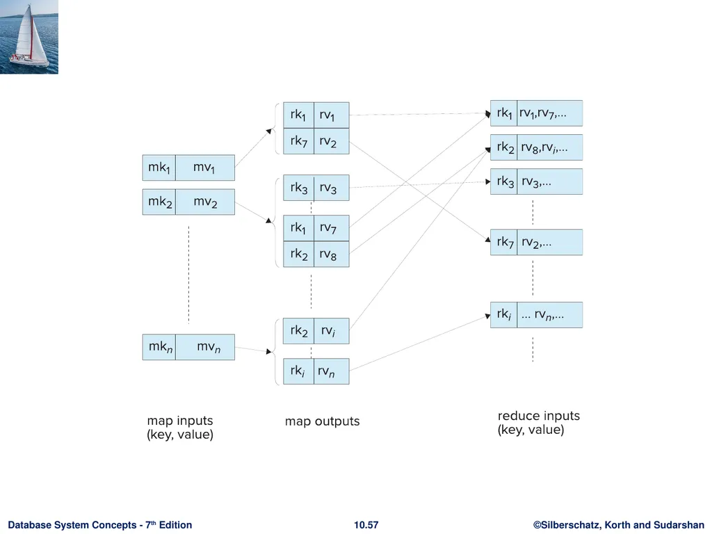
slide23. Schematic Flow of Keys and Values Flow of keys and values in a map reduce task<br>
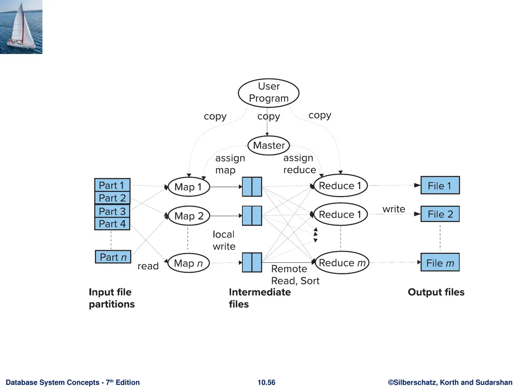
slide24. Parallel Processing of MapReduce Job<br>
slide25. Hadoop MapReduce Google pioneered map-reduce implementations that could run on thousands of machines (nodes), and transparently handle failures of machines
Hadoop is a widely used open source implementation of Map Reduce written in Java
Map and reduce functions can be written in several different languages, we use Java.
Input and output to map reduce systems such as Hadoop must be done in parallel
Google used GFS distributed file system
Hadoop uses Hadoop File System (HDFS),
Input files can be in several formats
Text/CSV
compressed representation such as Avro, ORC and Parquet
Hadoop also supports key-value stores such as Hbase, Cassandra, MongoDB, etc.<br>
slide26. Types in Hadoop Generic Mapper and Reducer interfaces both take four type arguments, that specify the types of the
input key, input value, output key and output value
Map class in next slide implements the Mapper interface
Map input key is of type LongWritable, i.e. a long integer
Map input value which is (all or part of) a document, is of type Text.
Map output key is of type Text, since the key is a word,
Map output value is of type IntWritable, which is an integer value.<br>
slide27. Hadoop Code in Java: Map Function public static class Map extends Mapper<LongWritable, Text, Text, IntWritable>
{
private final static IntWritable one = new IntWritable(1);
private Text word = new Text();
public void map(LongWritable key, Text value, Context context) throws IOException, InterruptedException
{
String line = value.toString();
StringTokenizer tokenizer = new StringTokenizer(line);
while (tokenizer.hasMoreTokens()) {
word.set(tokenizer.nextToken());
context.write(word, one);
}
}
}<br>
slide28. Hadoop Code in Java: Reduce Function public static class Reduce extends Reducer<Text, IntWritable, Text, IntWritable> {
public void reduce(Text key, Iterable<IntWritable> values, Context context) throws IOException, InterruptedException
{
int sum = 0;
for (IntWritable val : values) {
sum += val.get();
}
context.write(key, new IntWritable(sum));
}
}<br>
slide29. Hadoop Job Parameters The classes that contain the map and reduce functions for the job
Set by methods setMapperClass() and setReducerClass()
The types of the job’s output key and values
Set by methods setOutputKeyClass() and setOutputValueClass()
The input format of the job
Set by method job.setInputFormatClass()
Default input format in Hadoop is the TextInputFormat,
Map key whose value is a byte offset into the file, and
Map value is the contents of one line of the file
The directories where the input files are stored, and where the output files must be created
Set by addInputPath() and addOutputPath()
And many more parameters<br>
slide30. Hadoop Code in Java: Overall Program public class WordCount {
public static void main(String[] args) throws Exception {
Configuration conf = new Configuration();
Job job = new Job(conf, "wordcount");
job.setOutputKeyClass(Text.class);
job.setOutputValueClass(IntWritable.class);
job.setMapperClass(Map.class);
job.setReducerClass(Reduce.class);
job.setInputFormatClass(TextInputFormat.class);
job.setOutputFormatClass(TextOutputFormat.class);
FileInputFormat.addInputPath(job, new Path(args[0]));
FileOutputFormat.setOutputPath(job, new Path(args[1]));
job.waitForCompletion(true);
}
}<br>
slide31. Local Pre-Aggregation Combiners: perform partial aggregation to minimize network traffic
E.g., within machine
And/or at rack level
In Hadoop, reduce function is used by default if combiners are enabled
But alternative implementation of combiner can be specified if input and output types of reducers are different<br>
slide32. Map Reduce vs. Databases Map Reduce widely used for parallel processing
Google, Yahoo, and 100’s of other companies
Example uses: compute PageRank, build keyword indices, do data analysis of web click logs, ….
Allows procedural code in map and reduce functions
Allows data of any type
Many real-world uses of MapReduce cannot be expressed in SQL
But many computations are much easier to express in SQL
Map Reduce is cumbersome for writing simple queries<br>
slide33. Map Reduce vs. Databases (Cont.) Relational operations (select, project, join, aggregation, etc.) can be expressed using Map Reduce
SQL queries can be translated into Map Reduce infrastructure for execution
Apache Hive SQL, Apache Pig Latin, Microsoft SCOPE
Current generation execution engines support not only Map Reduce, but also other algebraic operations such as joins, aggregation, etc. natively.<br>
slide34. Beyond MapReduce: Algebraic Operations<br>
slide35. Algebraic Operations Current generation execution engines
natively support algebraic operations such as joins, aggregation, etc. natively.
Allow users to create their own algebraic operators
Support trees of algebraic operators that can be executed on multiple nodes in parallel
E.g. Apache Tez, Spark
Tex provides low level API; Hive on Tez compiles SQL to Tez
Spark provides more user-friendly API<br>
slide36. Algebraic Operations in Spark Resilient Distributed Dataset (RDD) abstraction
Collection of records that can be stored across multiple machines
RDDs can be created by applying algebraic operations on other RDDs
RDDs can be lazily computed when needed
Spark programs can be written in Java/Scala/R
Our examples are in Java
Spark makes use of Java 8 Lambda expressions; the code
s - > Arrays.asList(s.split(" ")).iterator()
defines unnamed function that takes argument s and executes the expression Arrays.asList(s.split(" ")).iterator() on the argument
Lambda functions are particularly convenient as arguments to map, reduce and other functions<br>
slide37. Word Count in Spark<br>
slide38. Algebraic Operations in Spark Algebraic operations in Spark are typically executed in parallel on multiple machines
With data partitioned across the machines
Algebraic operations are executed lazily, not immediately
Our preceding program creates an operator tree
Tree is executed only on specific functions such as saveAsTextFile() or collect()
Query optimization can be performed on tree before it is executed<br>
slide39. Spark DataFrames and DataSet RDDs in Spark can be typed in programs, but not dynamically
The DataSet type allows types to be specified dynamically
Row is a row type, with attribute names
In code below, attribute names/types of instructor and department are inferred from files read
Operations filter, join, groupBy, agg, etc defined on DataSet, and can execute in parallel
Dataset<Row> instructor = spark.read().parquet("..."); Dataset<Row> department = spark.read().parquet("..."); instructor.filter(instructor.col("salary").gt(100000)) .join(department, instructor.col("dept name") .equalTo(department.col("dept name"))) .groupBy(department.col("building")) .agg(count(instructor.col("ID")));<br>
slide40. Streaming Data<br>
slide41. Streaming Data and Applications Streaming data refers to data that arrives in a continuous fashion
Contrast to data-at-rest
Applications include:
Stock market: stream of trades
e-commerce site: purchases, searches
Sensors: sensor readings
Internet of things
Network monitoring data
Social media: tweets and posts can be viewed as a stream
Queries on streams can be very useful
Monitoring, alerts, automated triggering of actions<br>
slide42. Querying Streaming Data Windowing: Break up stream into windows, and queries are run on windows
Stream query languages support window operations
Windows may be based on time or tuples
Must figure out when all tuples in a window have been seen
Easy if stream totally ordered by timestamp
Punctuations specify that all future tuples have timestamp greater that some value
Continuous Queries: Queries written e.g. in SQL, output partial results based on stream seen so far; query results updated continuously
Have some applications, but can lead to flood of updates Approaches to querying streams:<br>
slide43. Querying Streaming Data (Cont.) Algebraic operators on streams:
Each operator consumes tuples from a stream and outputs tuples
Operators can be written e.g., in an imperative language
Operator may maintain state
Pattern matching:
Queries specify patterns, system detects occurrences of patterns and triggers actions
Complex Event Processing (CEP) systems
E.g., Microsoft StreamInsight, Flink CEP, Oracle Event Processing Approaches to querying streams (Cont.):<br>
slide44. Stream Processing Architectures Many stream processing systems are purely in-memory, and do not persist data
Lambda architecture: split stream into two, one output goes to stream processing system and the other to a database for storage
Easy to implement and widely used
But often leads to duplication of querying effort, once on streaming system and once in database<br>
slide45. Stream Extensions to SQL SQL Window functions described in Section 5.5.2
Streaming systems often support more window types
Tumbling window
E.g., hourly windows, windows don’t overlab
Hopping window
E.g., hourly window computed every 20 minutes
Sliding window
Window of specified size (based on timestamp interval or number of tuples) around each incoming tuple
Session window
Groups tuples based on user sessions<br>
slide46. Window Syntax in SQL Windowing syntax varies widely by system
E.g., in Azure Stream Analytics SQL:
select item, System.Timestamp as window end, sum(amount) from order timestamp by datetime group by itemid, tumblingwindow(hour, 1)
Aggregates are applied on windows
Result of windowing operation on a stream is a relation
Many systems support stream-relation joins
Stream-stream joins often require join conditions to specify bound on timestamp gap between matching tuples
E.g., tuples must be at most 30 minutes apart in timestamp<br>
slide47. Algebraic Operations on Streams Tuples in streams need to be routed to operators
Routing of streams using DAG and publish-subscribe representations
Used in Apache Storm and Apache Kafka respective<br>
slide48. Publish Subscribe Systems Publish-subscribe (pub-sub) systems provide convenient abstraction for processing streams
Tuples in a stream are published to a topic
Consumers subscribe to topic
Parallel pub-sub systems allow tuples in a topic to be partitioned across multiple machines
Apache Kafka is a popular parallel pub-sub system widely used to manage streaming data
More details in book<br>
slide49. Graph Databases<br>
slide50. Graph Data Model Graphs are a very general data model
ER model of an enterprise can be viewed as a graph
Every entity is a node
Every binary relationship is an edge
Ternary and higher degree relationships can be modelled as binary relationships<br>
slide51. Graph Data Model (Cont.) Graphs can be modelled as relations
node(ID, label, node_data)
edge(fromID, toID, label, edge_data)
Above representation too simplistic
Graph databases like Neo4J can provide a graph view of relational schema
Relations can be identified as representing either nodes or edges
Query languages for graph databases make it
easy to express queries requiring edge traversal
allow efficient algorithms to be used for evaluation<br>
slide52. Graph Data Model (Cont.) Suppose
Relations instructor and student are nodes, and
Relation advisor represents edges between instructors and student
Query in Neo4J: match (i:instructor)<-[:advisor]-(s:student) where i.dept name= 'Comp. Sci.’ return i.ID as ID, i.name as name, collect(s.name) as advisees
match clause matches nodes and edges in graphs
Recursive traversal of edges is also possible
Suppose prereq(course_id, prereq_id) is modeled as an edge
Transitive closure can be done as follows: match (c1:course)-[:prereq *1..]->(c2:course) return c1.course id, c2.course id<br>
slide53. Parallel Graph Processing Very large graphs (billions of nodes, trillions of edges)
Web graph: web pages are nodes, hyper links are edges
Social network graph: people are nodes, friend/follow links are edges
Two popular approaches for parallel processing on such graphs
Map-reduce and algebraic frameworks
Bulk synchronous processing (BSP) framework
Multiple iterations are required for any computations on graphs
Map-reduce/algebraic frameworks often have high overheads per iteration
BSP frameworks have much lower per-iteration overheads
Google’s Pregel system popularized the BSP framework
Apache Giraph is an open-source version of Pregel
Apache Spark’s GraphX component provides a Pregel-like API<br>
slide54. Bulk Synchronous Processing Each vertex (node) of a graph has data (state) associated with it
Vertices are partitioned across multiple machines, and state of node kept in-memory
Analogous to map() and reduce() functions, programmers provide methods to be executed for each node
Node method can send messages to or receive messages from neighboring nodes
Computation consists of multiple iterations, or supersteps
In each superstep
Nodes process received messages
Update their state, and
Send further messages or vote to halt
Computation ends when all nodes vote to halt, and there are no pending messages;<br>
slide55. End of Chapter 10<br>