OPTIMAL PROGRAME OF CAPITAL ACCUMIATION IN AMUTISECTOR ECONCWS Chakra - PDF document

1 OPTIMAL PROGRAME OF CAPITAL ACCUMIATION
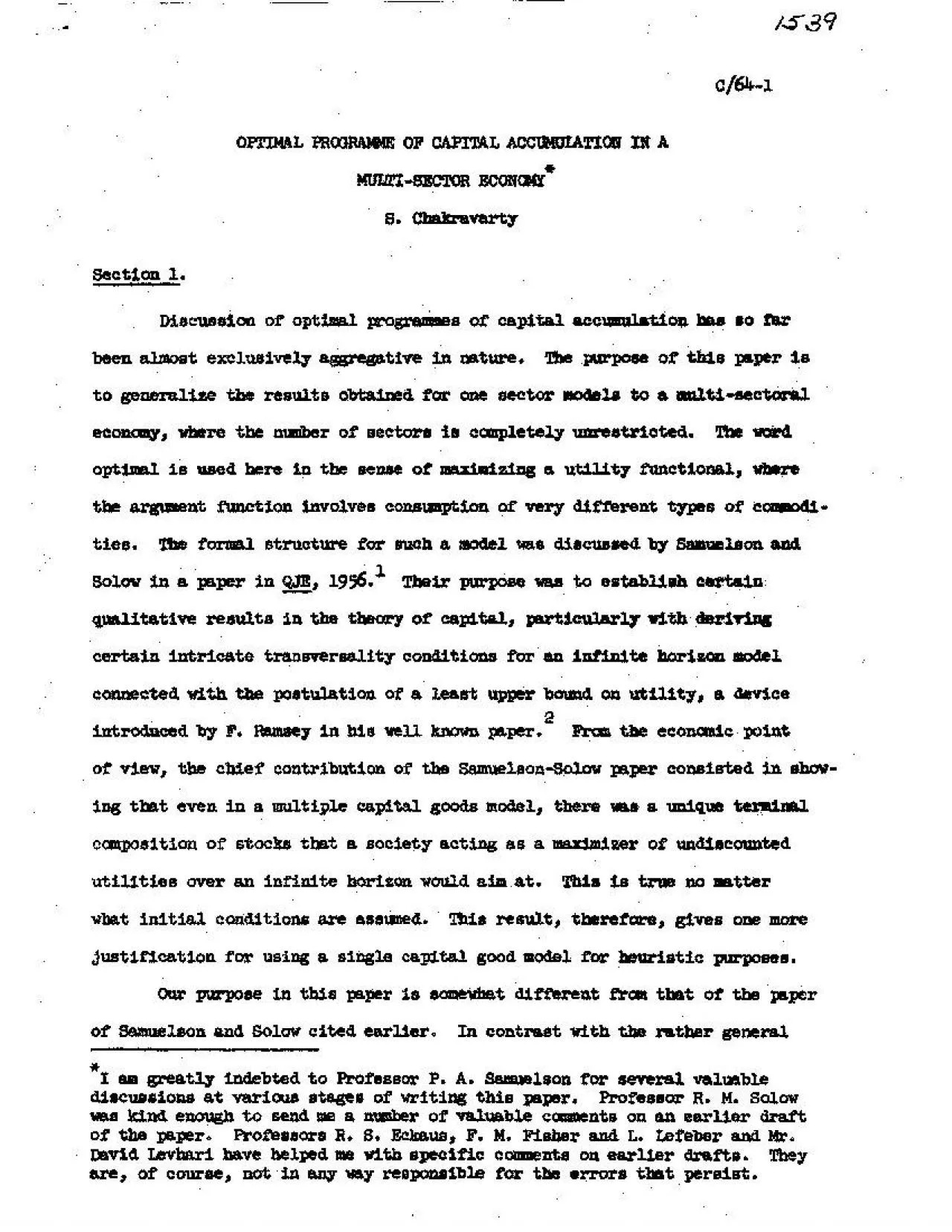
OPTIMAL PROGRAME OF CAPITAL ACCUMIATION IN A*MUTI-SECTOR ECONCWS. ChakravartySection 1.Discussion of optimal progranues of capital accumulation has so farbeen almost exclusively aggregative in nature. The purpose of this paper isto generalize the in a never firm the cost devise a -If.admissible functions are allowed to have piecewise continuous derivatives.For simple cases, one can hope to do something through simple trial anderror, although the problem is by no means trivial ev

2 en for a model withfew sectors.Our expli
en for a model withfew sectors.Our explicit solutions are obtained on the asuaption that no eesscapacity exists and that the utility function is a linear logritheic one.The Jatter assamption is much more easily relamble than the first. In factswe can indicate some more utility functions for which explicit solutionsmy be obtained. The absence of excess capacity is, however, a muchstronger assaption in this context. While there is no general reasonwhy an optimizing solution should ne

3 cessarily satisfy this condition, it isw
cessarily satisfy this condition, it isworthwhile making this assmption just to see how much it entails, andbecause ofalsoAthe assumption that an optimisingasozlution aWy in gesl be, exaetedto satisfy this condition for at least part of the planning horison.In our subsequent discussion we assume the planning horizon to be afinite one with appropriate initial and terminal conditions. Thus, we havea variational problem of the fixed end point variety. It should, however,be possible to

4 extend parts of our analysis to an infi
extend parts of our analysis to an infinite horizon model,if the utility functions are bounded, or suitable discount factorn are usedIsto ensure convergence of the functional. Whata 'suitable discount factorwill depend on the nature of technologically admissible growth partswhich are available to society. If the utility function is asemed to bebounded., it would be useful to make the additional assumption that the leastupper bound on utility is achieved for a finite vector of cons

5 umption. Thiswill rule out possible path
umption. Thiswill rule out possible pathologies in the undiscounted infinite horizonproblem. a WThere is no q.uestion that, from a fundamental conceptual point of view,adoption of a finite horizon for a planning model introduces an element ofdiscontinuity in the treatment of preferences for consumption within theplanning period and consumption beyond the planning period. Further, itis also true that there is an element of arbitrariness in the choice of ter-minal capital stock. This

6 arguent, however, loses part of its for
arguent, however, loses part of its force incertain cases, where the optimal consumption path is shown to be relativelyinsensitive to the choice, of terminal conditions. Despite these limitations,the use of a finite horizon model has a considerable amount of attractivenessfrom the point of view of constructing planning models, as many planners tendto think along such lines. c Is to assume (1) u + X the interpretation u) (b, past and -X C -the change if it is h S S + that the

7 x's are nonnegative. Thus, our Lagrangi
x's are nonnegative. Thus, our Lagrangian expreass on is now changedto the following one:U(c+ Z n (c -ln2) + Za (X -Za -S )+ Z (S -b x3 -e2) + I (S + h S u (X 32We have now the following first order condition:(1) j + X -X -0(2) ((I -A J), Xk) (bJ, Z) + It -0a ki(3 +h 'K + A -(5) -0(6) uj -0(7) Yrm -0A comparison with the earlier models will indicate that the set of optimisingconditions is now somewhat changed. But the qualitative structure of thesolutions is unchanged, as one wou

8 ld expect., Section 3.We shall consider
ld expect., Section 3.We shall consider the special case of a linear logarithmic utility fumc.Ttion, Our utility functional can now be written as / (Z pi log ci) dt.0Since we assume that there is no excess capacity, we can writeFor this cases we can derive the necessary Euler..Lagrange equations from thegeneralized Ramsey condition by putting u -p /C3.Alternatively, we canderive the Euler-Lagrange equations through direct substitution of x.'s for c a'0The latter procedure is the mo

9 re straight forward one and the sufficie
re straight forward one and the sufficiey of theEuler-Lagrange condition for a global maximum is directly proved in thi oaseby the simple Legendre condition of diminishing marginal utility. We *hall,therefore, use this straight forward derivation to indicate its simplifedcharacter0Here our functional gets transformed into the following expression:TZp log (xi -A -Abij)dt0T+I p log (xl Zalx -Zb j)0T+ f p2 log (x2 -Za23x: -Zb2')T+ p n ~ nlog (Y. Za njxj Zb' :.This meansT TZ (p± log c

10 i)dt -/ F (x, X2'.sx n oo*n)dt.Here xi's
i)dt -/ F (x, X2'.sx n oo*n)dt.Here xi's represent output levels, (a ) the matrix of current input require-ments and (bi) is the matrix of capital requirements per unit of output0The--13-0 3241 .n n 21-b -b1 -b1 A) PqHence the solution form a -17-we have nonnegative c(t) for 0 T. It should be added, however, that evenif ces were all to preserve nonnegativity for any It', a situation which wecannot guarantee in advance, there is no reason to think that x's will preservenonnegativ

11 ity for all it'. In fact, the discussion
ity for all it'. In fact, the discussion on the dynamic Ieontiefmodel following from the fundamental work of Dorfman, Samuelson and Solo6 wouldlead one to infer that the nonnegativity condition is violated for an infiniteT, save in special cases. For a finite horizon, we may be more lucky, buteven in that case, there is no easily applicable list that we can rely uponto ensure nonnegativity in advance. To ensure nonnegativity, we have to fallback on the more general model discussed

12 in Section 2 in this paper, As thediscus
in Section 2 in this paper, As thediscussion there indicates, computation of an optimal solution in that caseraises problems which have not been tackled in the mathematical literature inits proper generality,In addition to the linear logarithmic utility function, we can think ofa few other utility functions for which the above technique will yield readilycomputable solutions. First, we can assume that U -c 1 2 2...n whereots are constants. Since we are maximizing an expression Jdt,

13 this utilityfunction gives us a differe
this utilityfunction gives us a different optimizing solution from the one associated withp p log ci dt. This is obvious because fUdt admits only of arbitrary lineartransformations. The other case is a much simpler one, namely, the situationwhere the utility function is quadratic, with a negative definite quadraticform, Here, Euler equations are linear in the consumption levels, and hencethe analysis of the resulting time paths is much easiero -18-Section 4.Pontryagin' s method fo

14 r determining optimal controle can be ap
r determining optimal controle can be applied toour problem in a straightforward fashion on simple terminological adaptations.His problem is to determine the vector function u(t) which maximizes anTintegral f0 (x, u) dt where the x's and u' I are connected by differential0 dxequations such as dt -f(x, u) where f is a vector function conneted withvector variables x and u. This is the same problem as the one encountered inthe ordinary calculus of variations of maximizing an integral

15 subject to non-integrable constraints. A
subject to non-integrable constraints. As a special case, the solution to the simplestn..variable variational problem can be obtained from Pontryagin's maximum prin-ciple if dx a u where ut's are our control variables. Pontryagin allows"Wu to belong to a compact subset of a topological space.Now Pontryagin's procedure requires the introduction of a number ofauxiliary variables Ys 1** satisfying the conditiondVi -Z __.5_U-' m V .These variables are conjugate with variables..x .In fa

16 ct, it can be proved that tx. w N for 0
ct, it can be proved that tx. w N for 0 t T where N isconstant. Thus, if V's are interpreted as prices, this implies that the totalvalue of output at any point on the optimal path is a constant. This is thesame as the law of conservation of energy in classical mechanics when theHamiltonian does not involve time explicitly.Once the -ra are defined, Pontryagin' s procedure consists of maximizingnthe function H w ZV, f, with respect to the control varia bles us.In our case, the contro

17 l variables are c's. Thus, we have the f
l variables are c's. Thus, we have the followingproblemi '19.H(t) -T0 (p, log C) + (V, B 1(I -A)x) -(4 B o)T can be proved to be a constant for optimal solution to this class of problem.The optimal values for c a are obtained by putting aR/ac -0.On the other hand, we havedi nT1 Bl + '2 B2 +. ++ BniHence N -B (I -A)Hence, we have T(t) -e-B (I-A)) Q where Q is a vector of initial conditions,Once the Y's are known, insertion of Y's in the condition all/ac -o willgive us back the equat

18 ion for the optimal path obtained by cla
ion for the optimal path obtained by classical methods.The equations forYts indicate that they are independent of the utilityfunction used* Therefore, so long as the technology is the same, the solutionfor V's will be the same. Moreover, since the equation for Y's is always linearhomogeneous, thus, even in the general case where technology is non-linear, thesolution of I's is simpler than that of the state variables x's. However, inthe more general case this will be of only limited

19 help because the relevant par.tial deri
help because the relevant par.tial derivatives will not be constant and, hence, we would not be able to solvethe Its quite independently of the state variables x s.We may interpret the V's as the values assumed by the marginal utilitiesof different commodities above the optimal path and this will be in perfectcorrespondence with the equations described in the earlier section. Thecorrespondence is easily established if we note that p /ct are the relevantmarginal utilities of the di

20 fferent commodities for a linear logarit
fferent commodities for a linear logarithmic utilityfunction. is satisfied the general it is Footnotes (continued)9. Samelson, P. A., "Efficient lhths of Capital Ac I ulaion in Tser ofCalculus of Variations," in kthematical Methods in the Social Sol-ences, edited by Kenneth Adrow,8iimJ Irli flic deStanford University Press, 1959.10. Tbis should be distinguished from the Keynes-amsey oendition whichstates the saving rule:U(X) dt B -U(z) Ihere U(1 denotes mrginaldcutility of consuti

21 on, M denotes the rates of capital fONsa
on, M denotes the rates of capital fONsation, andB, the bliss level of utility. par a system of B3,6 me tions that doesnot involve tim exli citly, an e mais the other Ros 0eins ofan infinite horizon and a least g er bont iR&y, the Busy eondi-tion can be shown to imply the Kynes-Rmey c=dities quoted here.11. Cominre Solow's conjectwe in Footnote 18, p. 49, of SoloV, "Cmpti-tive Valuations in ryneunio iontief Model," a l999, pp. 30-*53o22 Fermally, the condition, can be witten as fol

22 low.:(1) 8F AF (2)If the system is time
low.:(1) 8F AF (2)If the system is time independent, the expressions within the parenthesesin (2) are constant.13. The Legendre-Clebech condition is that F 0 wben we have a problemof maximizingTF (k, Io t) dt. For the n variable case, there is a0natural generalization in view of the negative definiteness of the rele-vant Hessian matrix.14. Bellman, R. Adaptive Control Processes.15. Radner, R., Notes on the Theory of 'Planning, Athens, 1963 has alsoused a linar logarithmic utility f

23 unction in connection with a oampletelyd
unction in connection with a oampletelydifferent model of technology. He may also adopt the convention from adnerthat whenever some a- 0 by definition since the conodity cannAot beused for consumption, the corresponding pi 0, with the stipulation that0 log 0. a 0. Footxots (co&Atmed)16. Dcifrmn, R,,, samasis=, P., and Ro Bcoov Linear Dro'su±gadEoaoAns~lo~oCharter' 3117. Pontrysgla, L. 8, $et, a]. Lb. I t ca3 MWOVY Of 29!pt,.l PomosspInterselene PibIs~s Ince, L%20 the prooedreUnive