CS 5600 Computer Systems Storage Devices Hard

slide1. CS 5600Computer Systems Storage Devices<br>
slide2. Hard Drives
RAID
SSD 2<br>
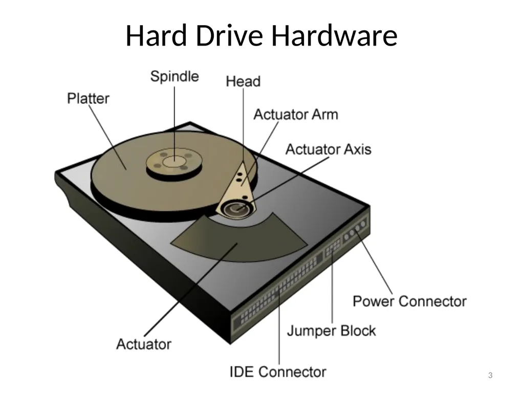
slide3. Hard Drive Hardware 3<br>
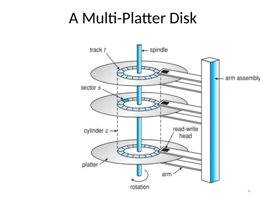
slide4. A Multi-Platter Disk 4<br>
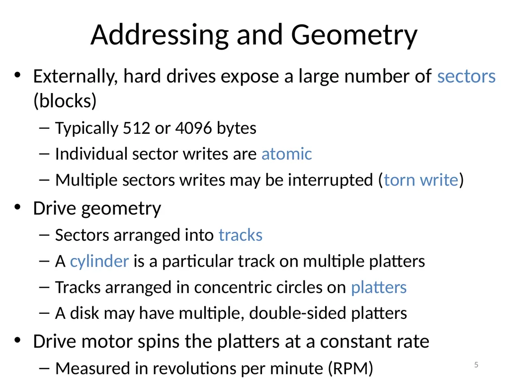
slide5. Addressing and Geometry Externally, hard drives expose a large number of sectors (blocks)
Typically 512 or 4096 bytes
Individual sector writes are atomic
Multiple sectors writes may be interrupted (torn write)
Drive geometry
Sectors arranged into tracks
A cylinder is a particular track on multiple platters
Tracks arranged in concentric circles on platters
A disk may have multiple, double-sided platters
Drive motor spins the platters at a constant rate
Measured in revolutions per minute (RPM) 5<br>
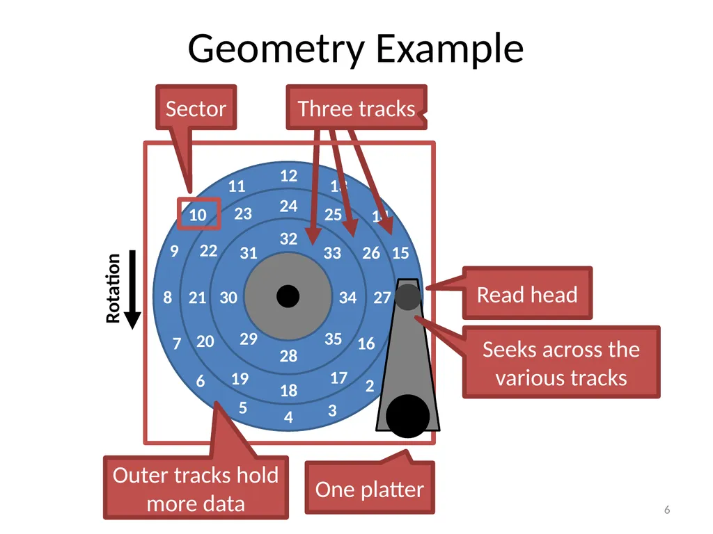
slide6. Geometry Example 6 Rotation Three tracks One platter Sector Outer tracks hold more data Read head Seeks across the various tracks<br>
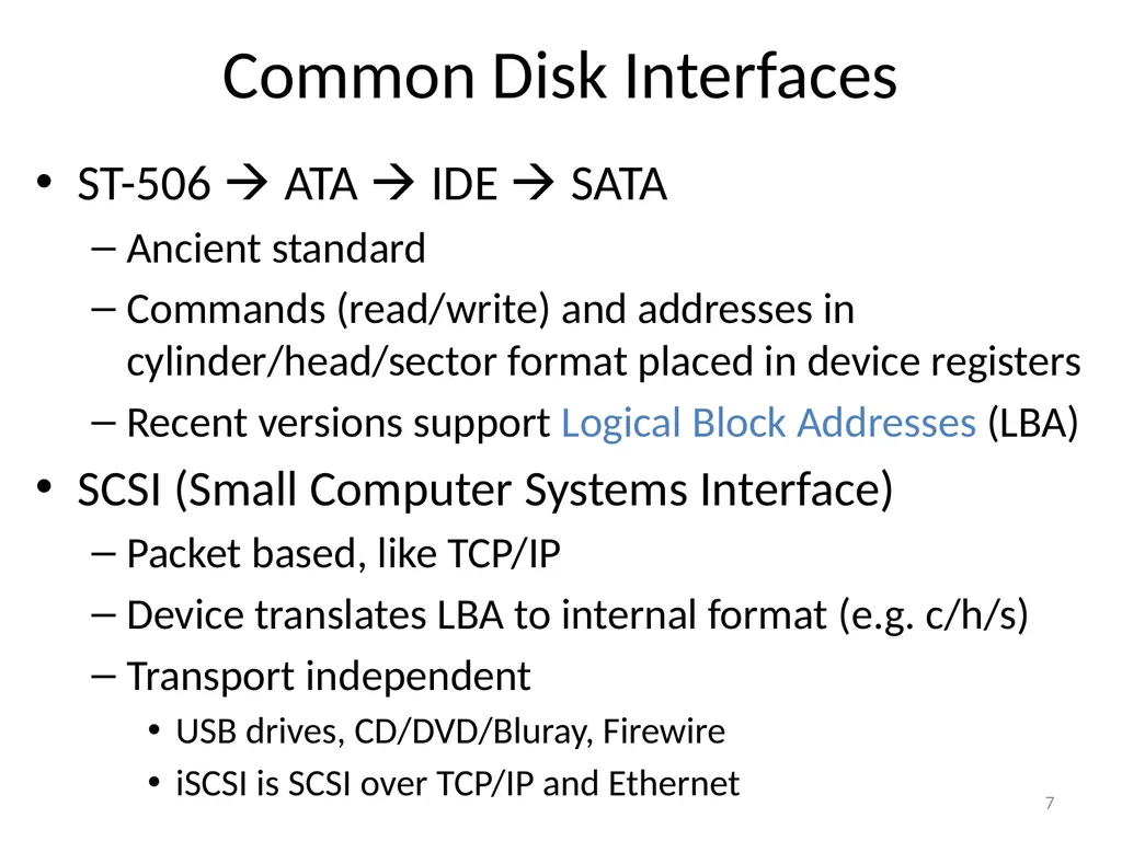
slide7. Common Disk Interfaces ST-506  ATA  IDE  SATA
Ancient standard
Commands (read/write) and addresses in cylinder/head/sector format placed in device registers
Recent versions support Logical Block Addresses (LBA)
SCSI (Small Computer Systems Interface)
Packet based, like TCP/IP
Device translates LBA to internal format (e.g. c/h/s)
Transport independent
USB drives, CD/DVD/Bluray, Firewire
iSCSI is SCSI over TCP/IP and Ethernet 7<br>
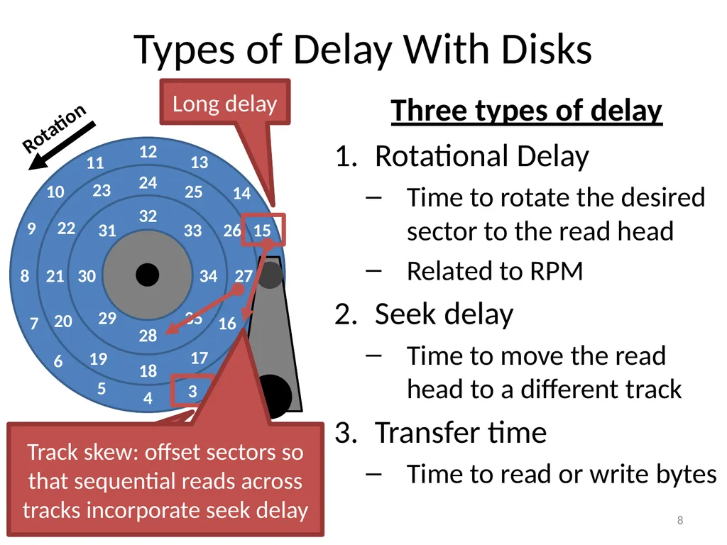
slide8. Types of Delay With Disks 8 Three types of delay
Rotational Delay
Time to rotate the desired sector to the read head
Related to RPM
Seek delay
Time to move the read head to a different track
Transfer time
Time to read or write bytes Rotation Short delay Long delay Track skew: offset sectors so that sequential reads across tracks incorporate seek delay<br>
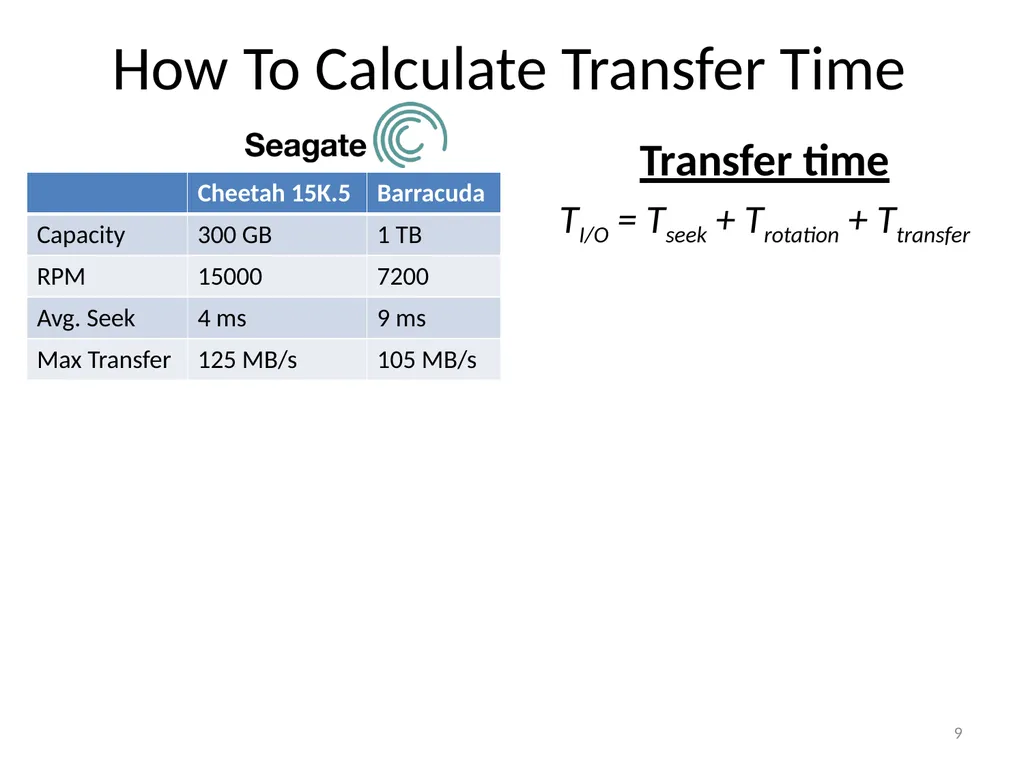
slide9. How To Calculate Transfer Time 9 Transfer time
TI/O = Tseek + Trotation + Ttransfer<br>
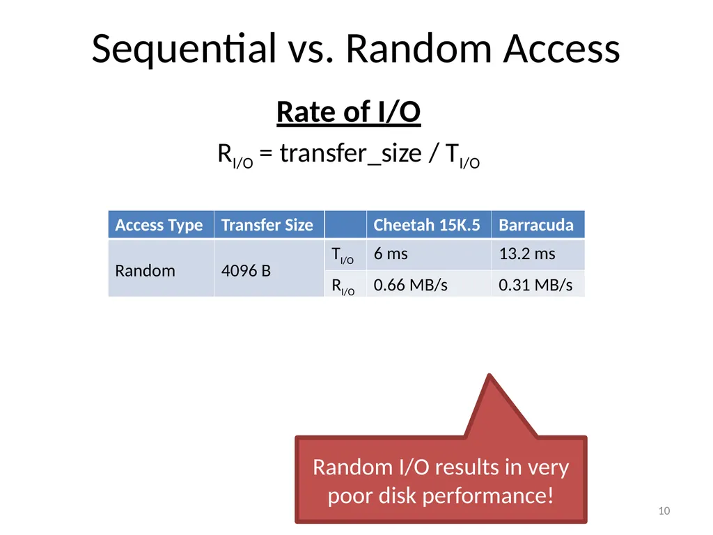
slide10. Sequential vs. Random Access Rate of I/O
RI/O = transfer_size / TI/O 10 Random I/O results in very poor disk performance!<br>
slide11. Caching Many disks incorporate caches (track buffer)
Small amount of RAM (8, 16, or 32 MB)
Read caching
Reduces read delays due to seeking and rotation
Write caching
Write back cache: drive reports that writes are complete after they have been cached
Possibly dangerous feature. Why?
Write through cache: drive reports that writes are complete after they have been written to disk
Today, some disks include flash memory for persistent caching (hybrid drives) 11<br>
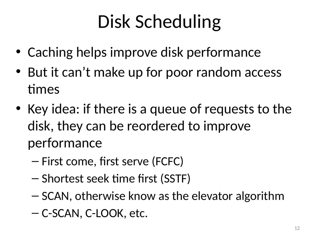
slide12. Disk Scheduling Caching helps improve disk performance
But it can’t make up for poor random access times
Key idea: if there is a queue of requests to the disk, they can be reordered to improve performance
First come, first serve (FCFC)
Shortest seek time first (SSTF)
SCAN, otherwise know as the elevator algorithm
C-SCAN, C-LOOK, etc. 12<br>
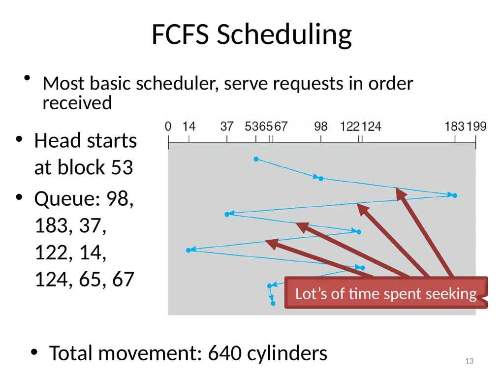
slide13. FCFS Scheduling Head starts at block 53
Queue: 98, 183, 37, 122, 14, 124, 65, 67 13 Total movement: 640 cylinders Lot’s of time spent seeking Most basic scheduler, serve requests in order received<br>
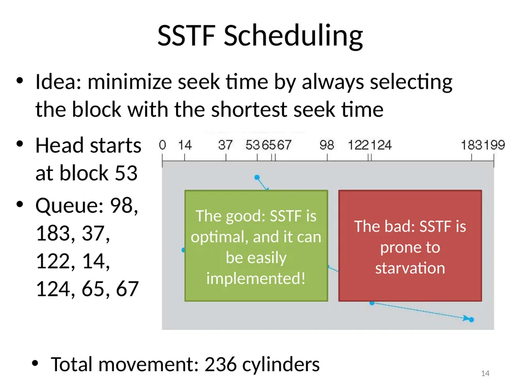
slide14. SSTF Scheduling Idea: minimize seek time by always selecting the block with the shortest seek time 14 Total movement: 236 cylinders Head starts at block 53
Queue: 98, 183, 37, 122, 14, 124, 65, 67 The good: SSTF is optimal, and it can be easily implemented! The bad: SSTF is prone to starvation<br>
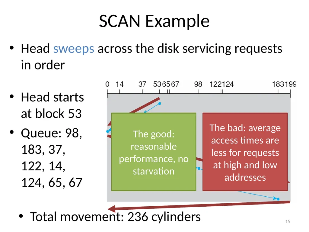
slide15. SCAN Example Head sweeps across the disk servicing requests in order 15 Total movement: 236 cylinders Head starts at block 53
Queue: 98, 183, 37, 122, 14, 124, 65, 67 The good: reasonable performance, no starvation The bad: average access times are less for requests at high and low addresses<br>
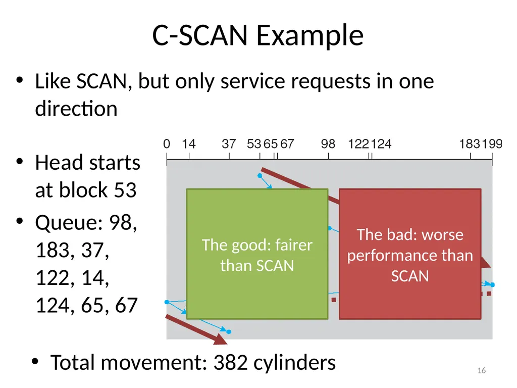
slide16. C-SCAN Example Like SCAN, but only service requests in one direction 16 Total movement: 382 cylinders Head starts at block 53
Queue: 98, 183, 37, 122, 14, 124, 65, 67 The good: fairer than SCAN The bad: worse performance than SCAN<br>
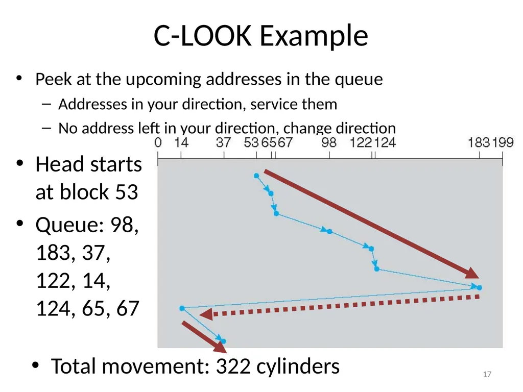
slide17. C-LOOK Example Peek at the upcoming addresses in the queue
Addresses in your direction, service them
No address left in your direction, change direction 17 Total movement: 322 cylinders Head starts at block 53
Queue: 98, 183, 37, 122, 14, 124, 65, 67<br>
slide18. Implementing Disk Scheduling We have talked about several scheduling problems that take place in the kernel
Process scheduling
Page swapping
Where should disk scheduling be implemented?
OS scheduling
OS can implement SSTF or LOOK by ordering the queue by LBA
However, the OS cannot account for rotation delay
On-disk scheduling
Disk knows the exact position of the head and platters
Can implement more advanced schedulers (SPTF)
But, requires specialized hardware and drivers 18<br>
slide19. Command Queuing Feature where a disk stores a queue of pending read/write requests
Called Native Command Queuing (NCQ) in SATA
Disk may reorder items in the queue to improve performance
E.g. batch operations to close sectors/tracks
Supported by SCSI and modern SATA drives
Tagged command queuing: allows the host to place constraints on command re-ordering 19<br>
slide20. Hard Drives
RAID
SSD 20<br>
slide21. Beyond Single Disks Hard drives are great devices
Relatively fast, persistent storage
Shortcomings:
How to cope with disk failure?
Mechanical parts break over time
Sectors may become silently corrupted
Capacity is limited
Managing files across multiple physical devices is cumbersome
Can we make 10x 1 TB drives look like a 10 TB drive? 21<br>
slide22. Redundant Array of Inexpensive Disks RAID: use multiple disks to create the illusion of a large, faster, more reliable disk
Externally, RAID looks like a single disk
i.e. RAID is transparent
Data blocks are read/written as usual
No need for software to explicitly manage multiple disks or perform error checking/recovery
Internally, RAID is a complex computer system
Disks managed by a dedicated CPU + software
RAM and non-volatile memory
Many different configuration options (RAID levels) 22<br>
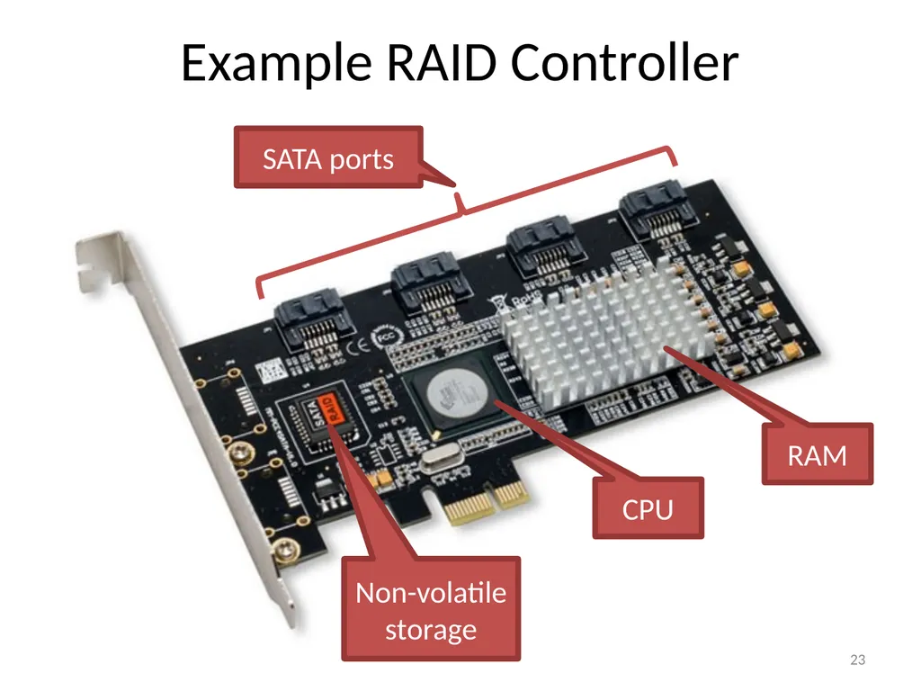
slide23. Example RAID Controller 23 SATA ports CPU RAM Non-volatile storage<br>
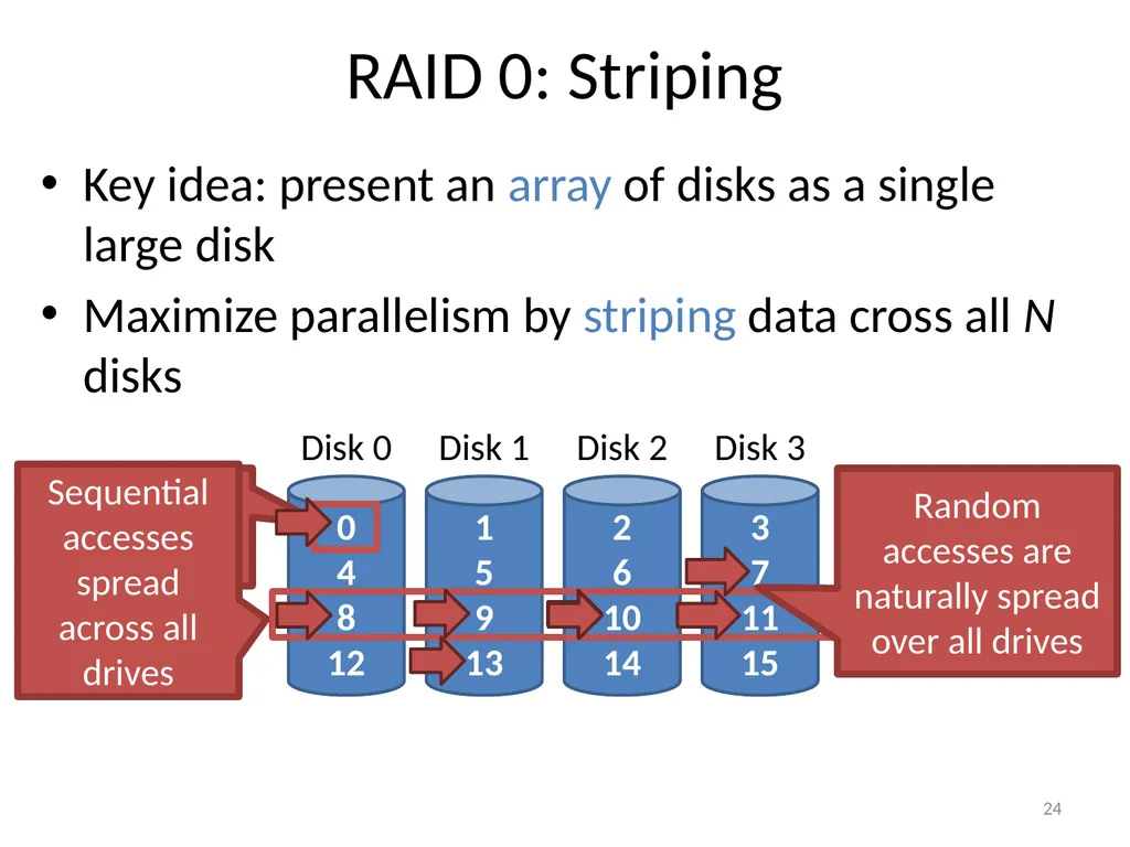
slide24. RAID 0: Striping Key idea: present an array of disks as a single large disk
Maximize parallelism by striping data cross all N disks 24 Stripe Data block = 512 bytes Random accesses are naturally spread over all drives Sequential accesses spread across all drives<br>
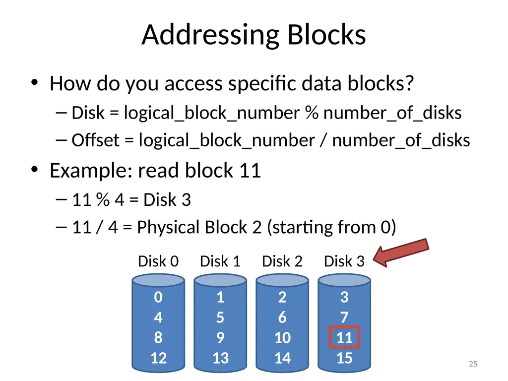
slide25. Addressing Blocks How do you access specific data blocks?
Disk = logical_block_number % number_of_disks
Offset = logical_block_number / number_of_disks
Example: read block 11
11 % 4 = Disk 3
11 / 4 = Physical Block 2 (starting from 0) 25<br>
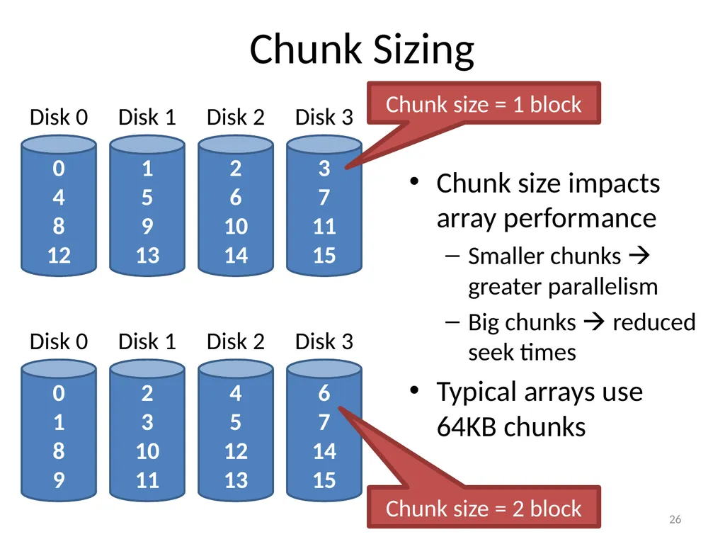
slide26. Chunk Sizing 26 Chunk size = 1 block Chunk size = 2 block Chunk size impacts array performance
Smaller chunks  greater parallelism
Big chunks  reduced seek times
Typical arrays use 64KB chunks<br>
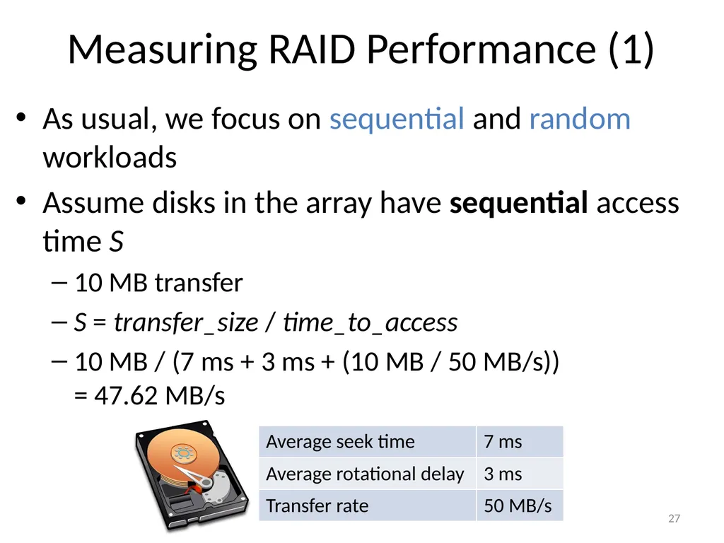
slide27. Measuring RAID Performance (1) As usual, we focus on sequential and random workloads
Assume disks in the array have sequential access time S
10 MB transfer
S = transfer_size / time_to_access
10 MB / (7 ms + 3 ms + (10 MB / 50 MB/s)) = 47.62 MB/s 27<br>
slide28. Measuring RAID Performance (2) As usual, we focus on sequential and random workloads
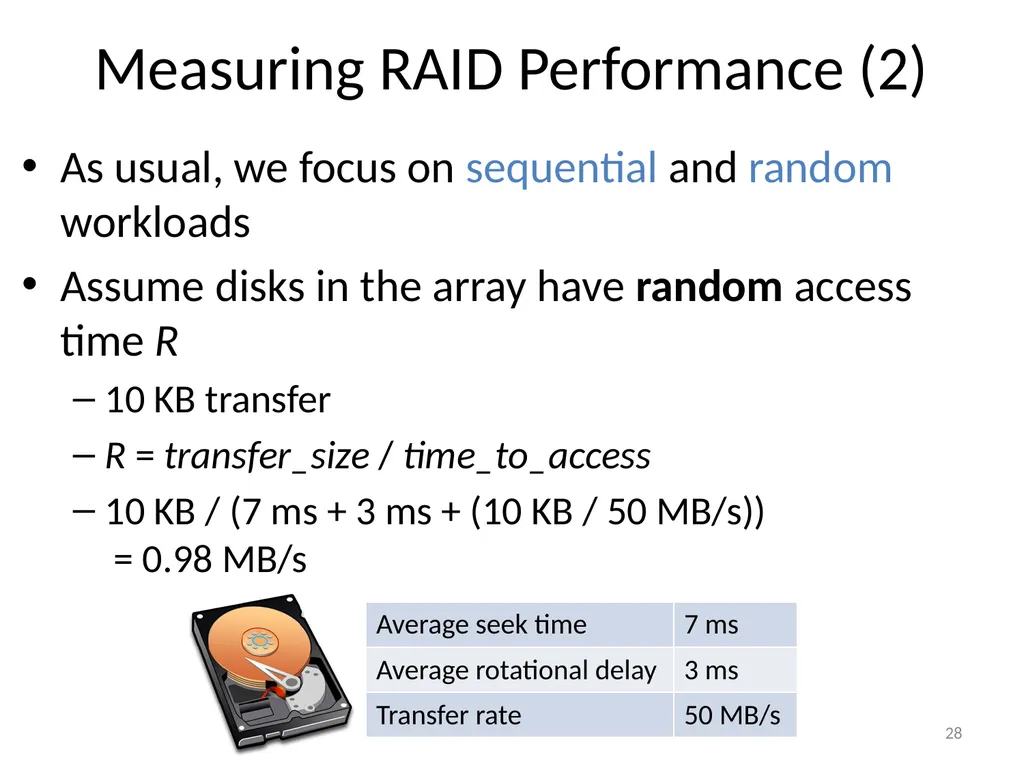
Assume disks in the array have random access time R
10 KB transfer
R = transfer_size / time_to_access
10 KB / (7 ms + 3 ms + (10 KB / 50 MB/s))  = 0.98 MB/s 28<br>
slide29. Analysis of RAID 0 Capacity: N
All space on all drives can be filled with data
Reliability: 0
If any drive fails, data is permanently lost
Sequential read and write: N * S
Full parallelization across drives
Random read and write: N * R
Full parallelization across all drives 29<br>
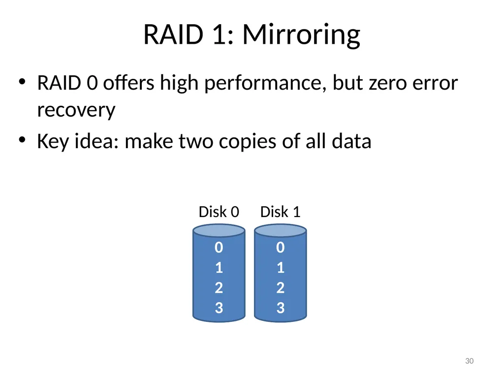
slide30. RAID 1: Mirroring 30 RAID 0 offers high performance, but zero error recovery
Key idea: make two copies of all data<br>
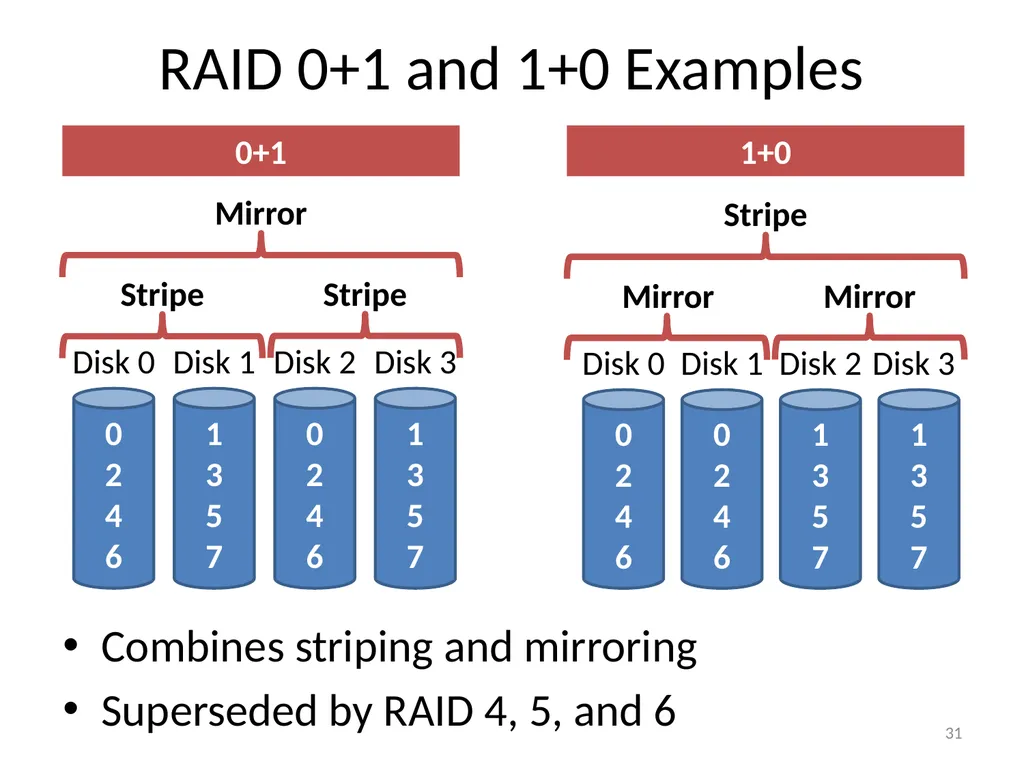
slide31. RAID 0+1 and 1+0 Examples 31 Combines striping and mirroring
Superseded by RAID 4, 5, and 6 0+1 1+0<br>
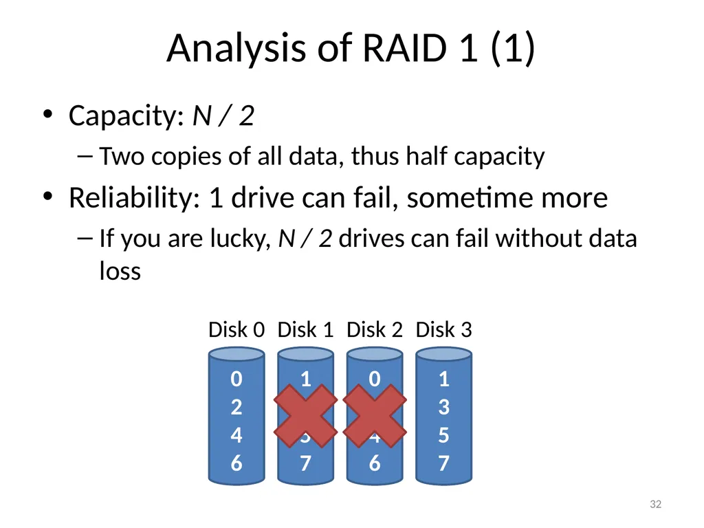
slide32. Analysis of RAID 1 (1) Capacity: N / 2
Two copies of all data, thus half capacity
Reliability: 1 drive can fail, sometime more
If you are lucky, N / 2 drives can fail without data loss 32<br>
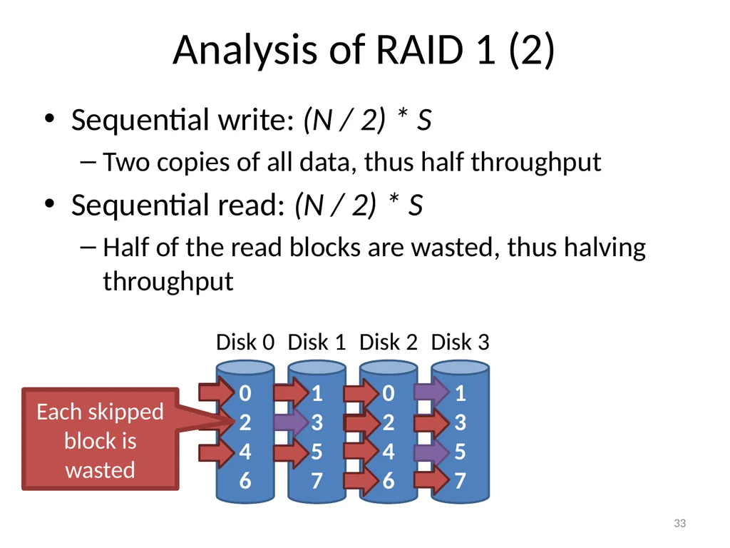
slide33. Analysis of RAID 1 (2) Sequential write: (N / 2) * S
Two copies of all data, thus half throughput
Sequential read: (N / 2) * S
Half of the read blocks are wasted, thus halving throughput 33 Each skipped block is wasted<br>
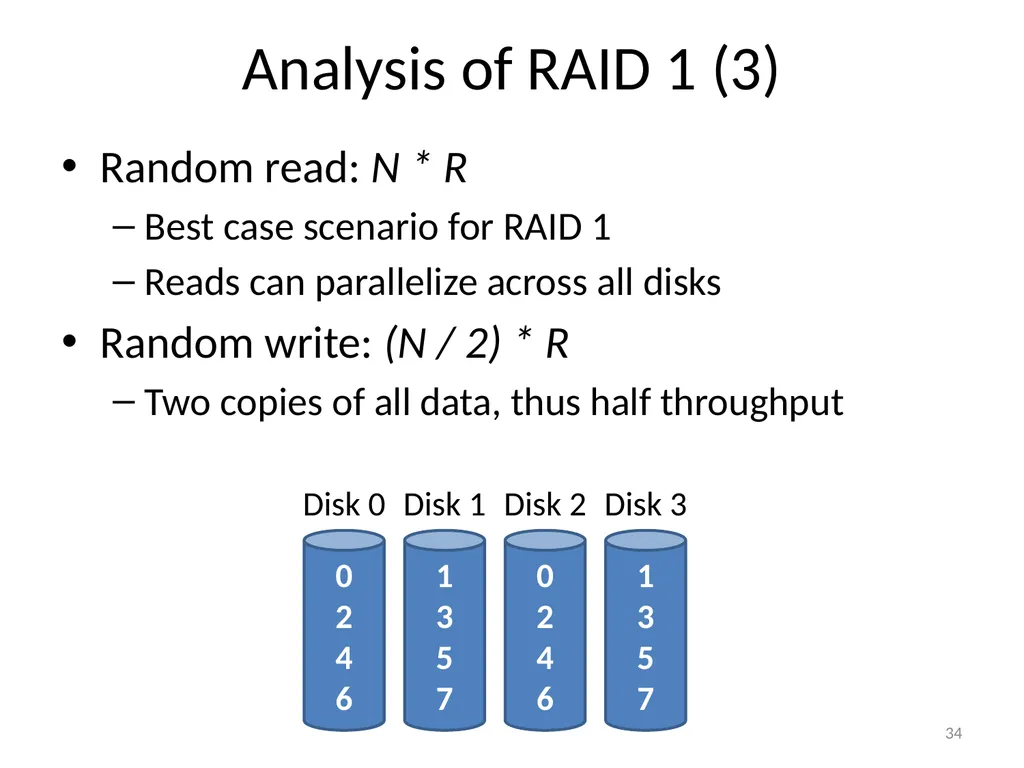
slide34. Analysis of RAID 1 (3) Random read: N * R
Best case scenario for RAID 1
Reads can parallelize across all disks
Random write: (N / 2) * R
Two copies of all data, thus half throughput 34<br>
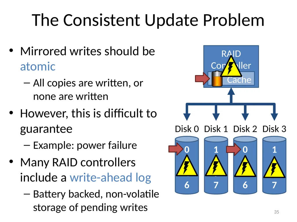
slide35. The Consistent Update Problem Mirrored writes should be atomic
All copies are written, or none are written
However, this is difficult to guarantee
Example: power failure
Many RAID controllers include a write-ahead log
Battery backed, non-volatile storage of pending writes 35 RAID Controller Cache<br>
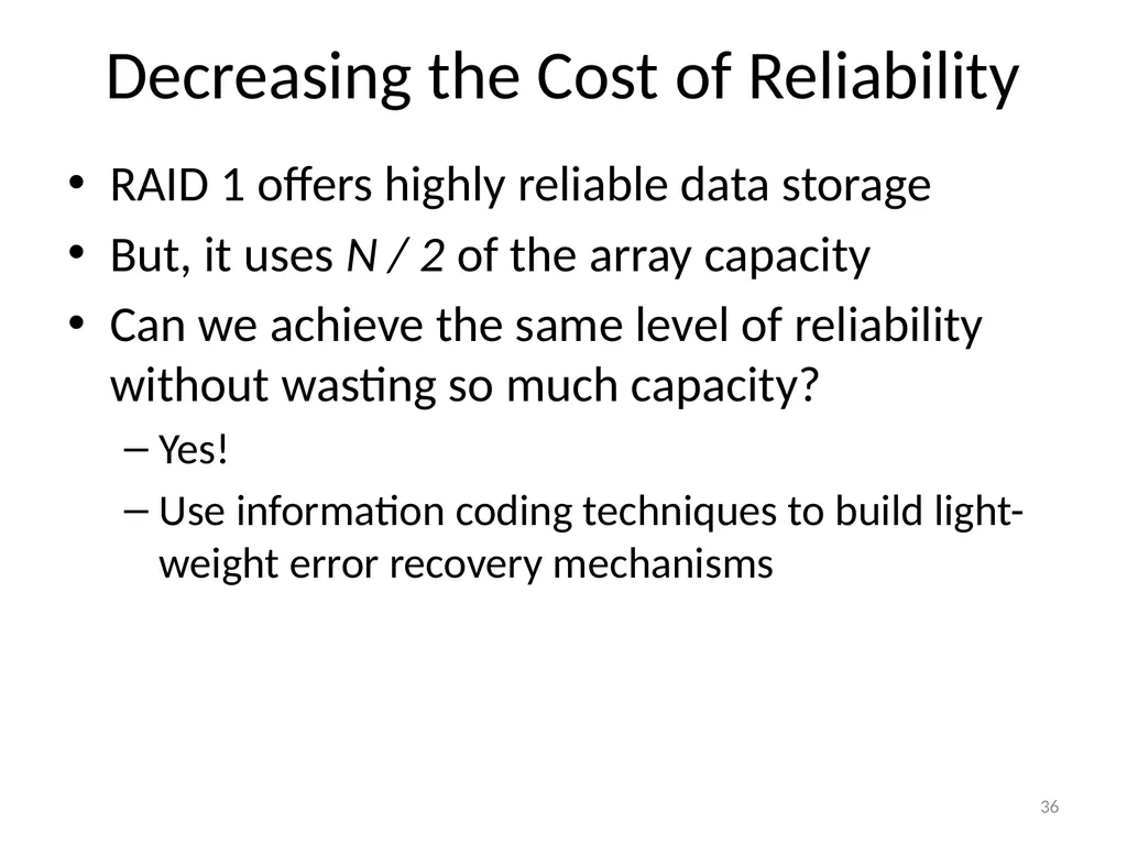
slide36. Decreasing the Cost of Reliability RAID 1 offers highly reliable data storage
But, it uses N / 2 of the array capacity
Can we achieve the same level of reliability without wasting so much capacity?
Yes!
Use information coding techniques to build light-weight error recovery mechanisms 36<br>
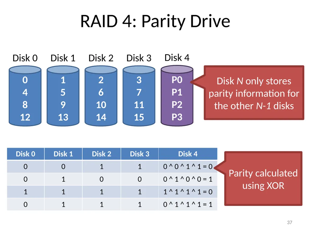
slide37. RAID 4: Parity Drive 37 Disk N only stores parity information for the other N-1 disks Parity calculated using XOR<br>
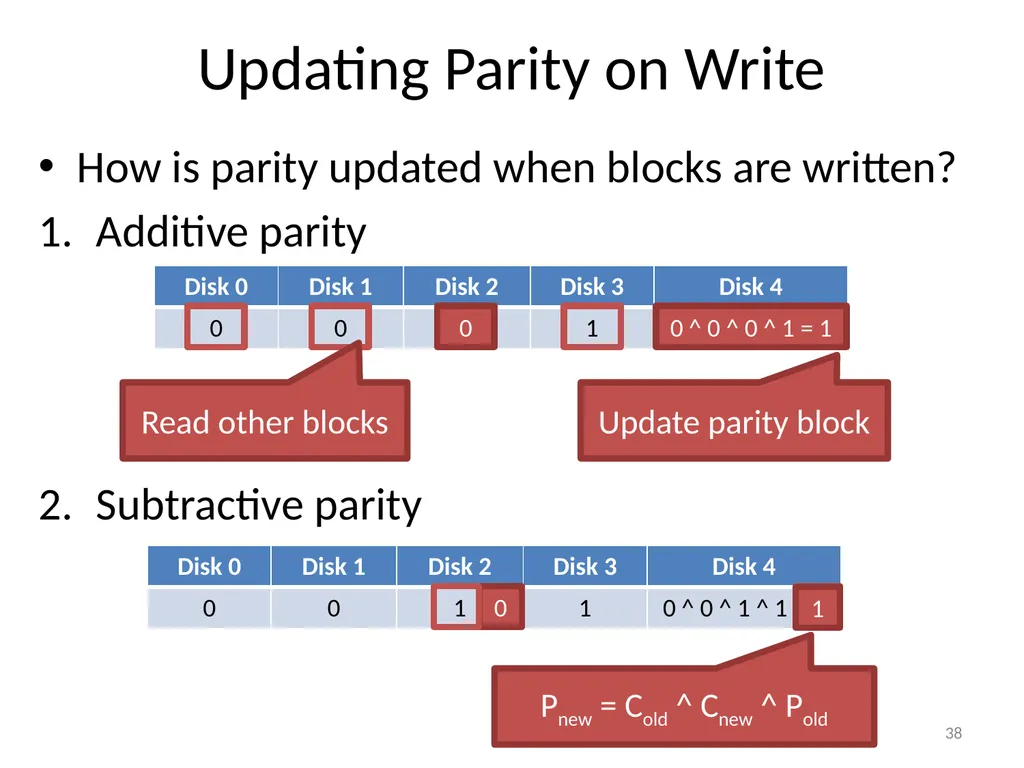
slide38. Updating Parity on Write How is parity updated when blocks are written?
Additive parity 38 Subtractive parity 0 0 ^ 0 ^ 0 ^ 1 = 1 Read other blocks Update parity block 0 1 Pnew = Cold ^ Cnew ^ Pold<br>
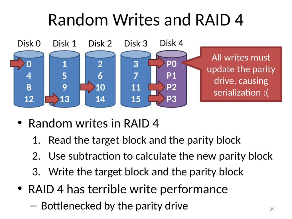
slide39. Random Writes and RAID 4 39 Random writes in RAID 4
Read the target block and the parity block
Use subtraction to calculate the new parity block
Write the target block and the parity block
RAID 4 has terrible write performance
Bottlenecked by the parity drive All writes must update the parity drive, causing serialization :(<br>
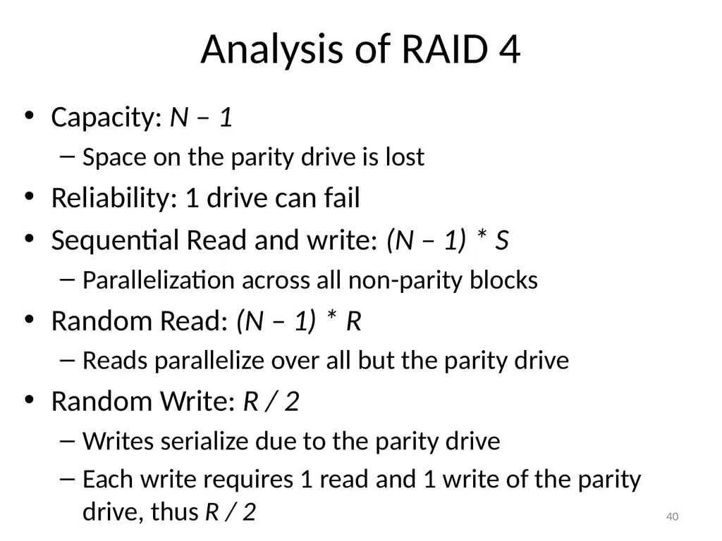
slide40. Analysis of RAID 4 Capacity: N – 1
Space on the parity drive is lost
Reliability: 1 drive can fail
Sequential Read and write: (N – 1) * S
Parallelization across all non-parity blocks
Random Read: (N – 1) * R
Reads parallelize over all but the parity drive
Random Write: R / 2
Writes serialize due to the parity drive
Each write requires 1 read and 1 write of the parity drive, thus R / 2 40<br>
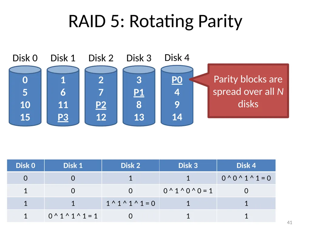
slide41. RAID 5: Rotating Parity 41 Parity blocks are spread over all N disks<br>
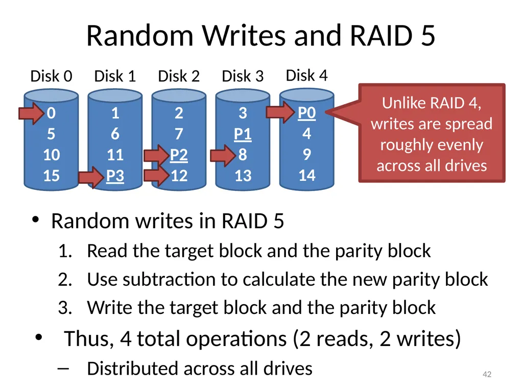
slide42. Random Writes and RAID 5 Random writes in RAID 5
Read the target block and the parity block
Use subtraction to calculate the new parity block
Write the target block and the parity block
Thus, 4 total operations (2 reads, 2 writes)
Distributed across all drives 42 Unlike RAID 4, writes are spread roughly evenly across all drives<br>
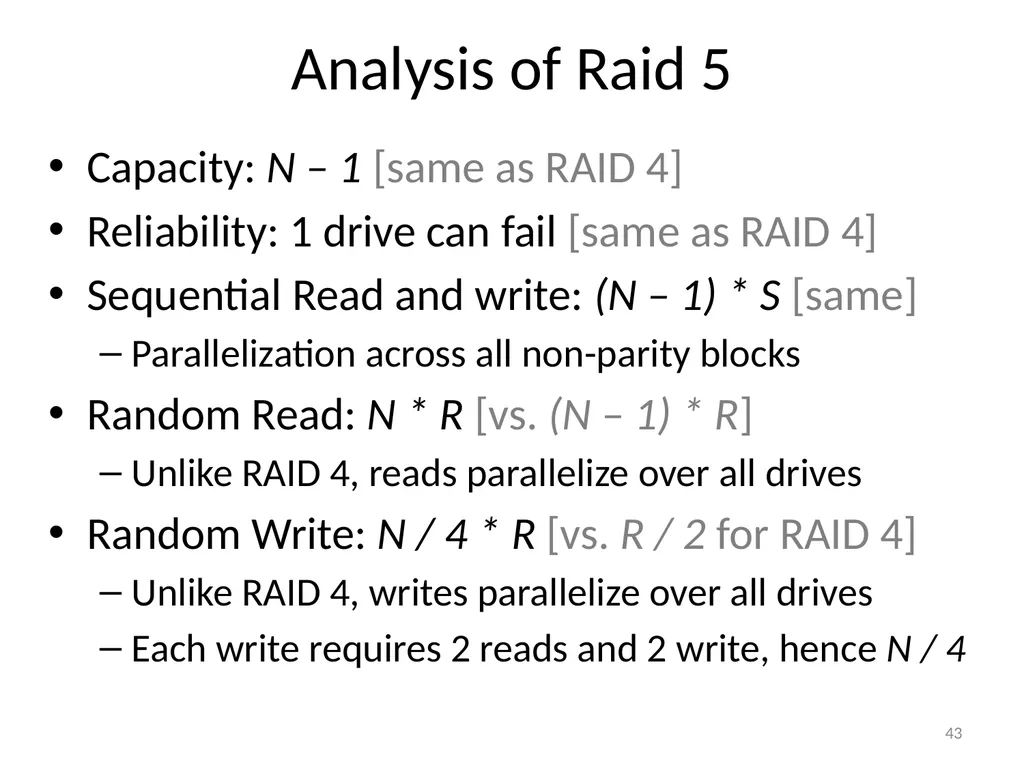
slide43. Analysis of Raid 5 Capacity: N – 1 [same as RAID 4]
Reliability: 1 drive can fail [same as RAID 4]
Sequential Read and write: (N – 1) * S [same]
Parallelization across all non-parity blocks
Random Read: N * R [vs. (N – 1) * R]
Unlike RAID 4, reads parallelize over all drives
Random Write: N / 4 * R [vs. R / 2 for RAID 4]
Unlike RAID 4, writes parallelize over all drives
Each write requires 2 reads and 2 write, hence N / 4 43<br>
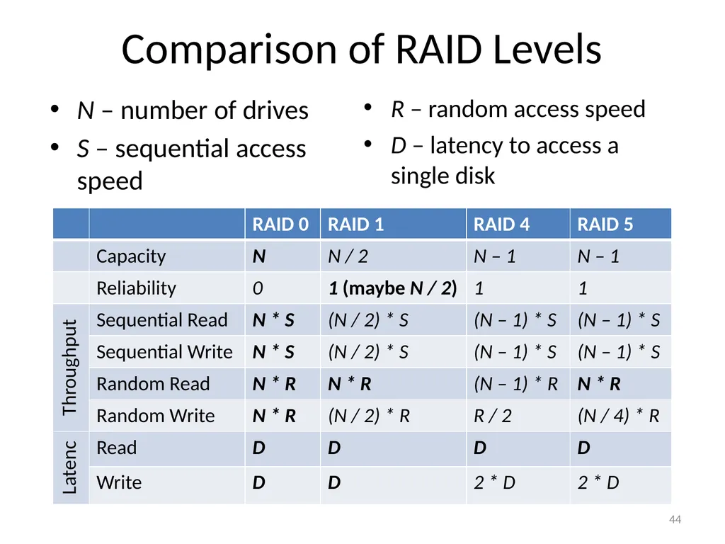
slide44. Comparison of RAID Levels 44 N – number of drives
S – sequential access speed R – random access speed
D – latency to access a single disk<br>
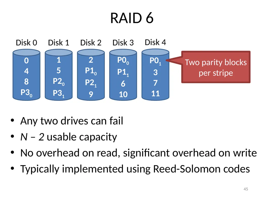
slide45. RAID 6 Any two drives can fail
N – 2 usable capacity
No overhead on read, significant overhead on write
Typically implemented using Reed-Solomon codes 45 Two parity blocks per stripe<br>
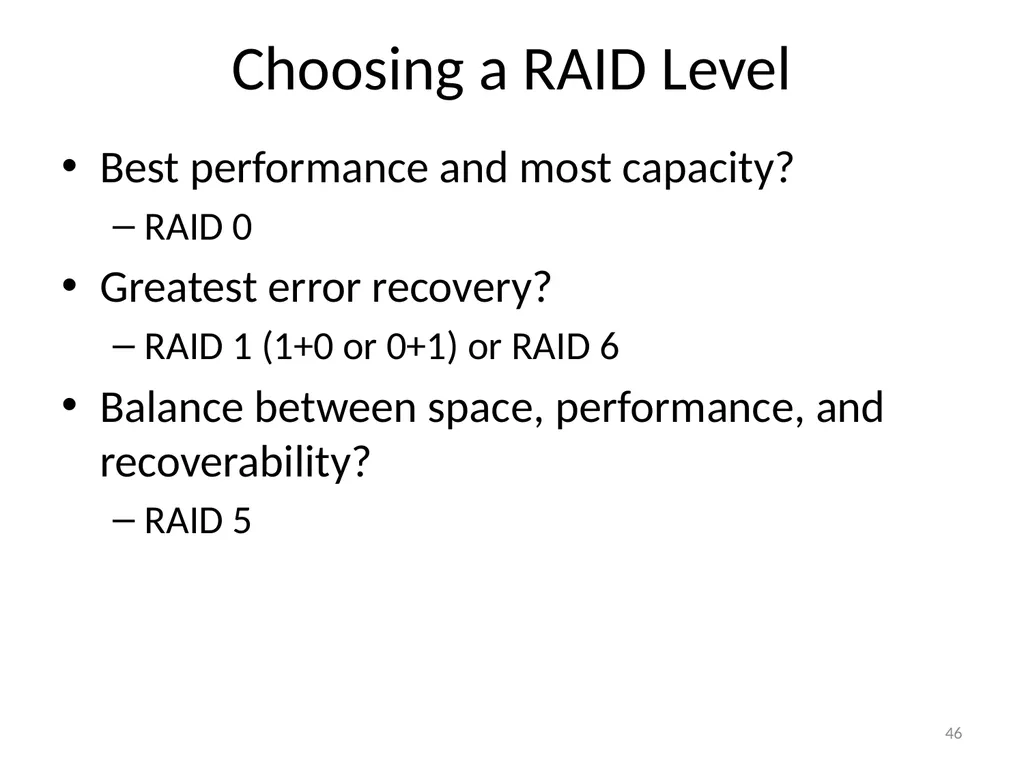
slide46. Choosing a RAID Level Best performance and most capacity?
RAID 0
Greatest error recovery?
RAID 1 (1+0 or 0+1) or RAID 6
Balance between space, performance, and recoverability?
RAID 5 46<br>
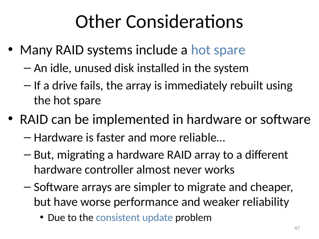
slide47. Other Considerations Many RAID systems include a hot spare
An idle, unused disk installed in the system
If a drive fails, the array is immediately rebuilt using the hot spare
RAID can be implemented in hardware or software
Hardware is faster and more reliable…
But, migrating a hardware RAID array to a different hardware controller almost never works
Software arrays are simpler to migrate and cheaper, but have worse performance and weaker reliability
Due to the consistent update problem 47<br>
slide48. Hard Drives
RAID
SSD 48<br>
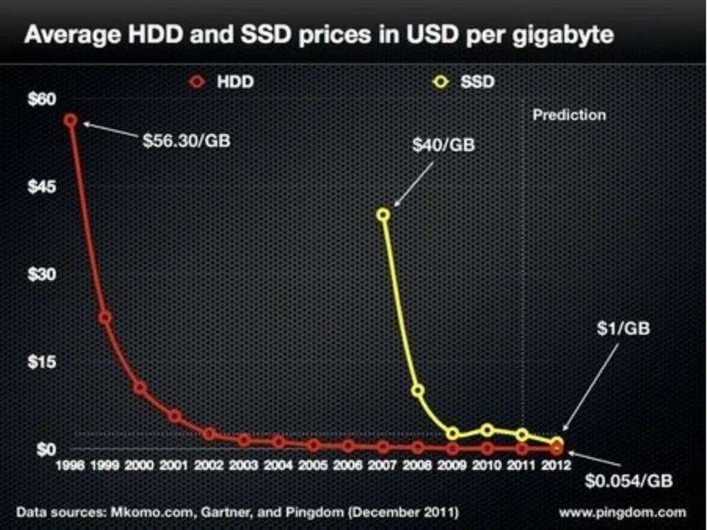
slide49. Beyond Spinning Disks Hard drives have been around since 1956
The cheapest way to store large amounts of data
Sizes are still increasing rapidly
However, hard drives are typically the slowest component in most computers
CPU and RAM operate at GHz
PCI-X and Ethernet are GB/s
Hard drives are not suitable for mobile devices
Fragile mechanical components can break
The disk motor is extremely power hungry 49<br>
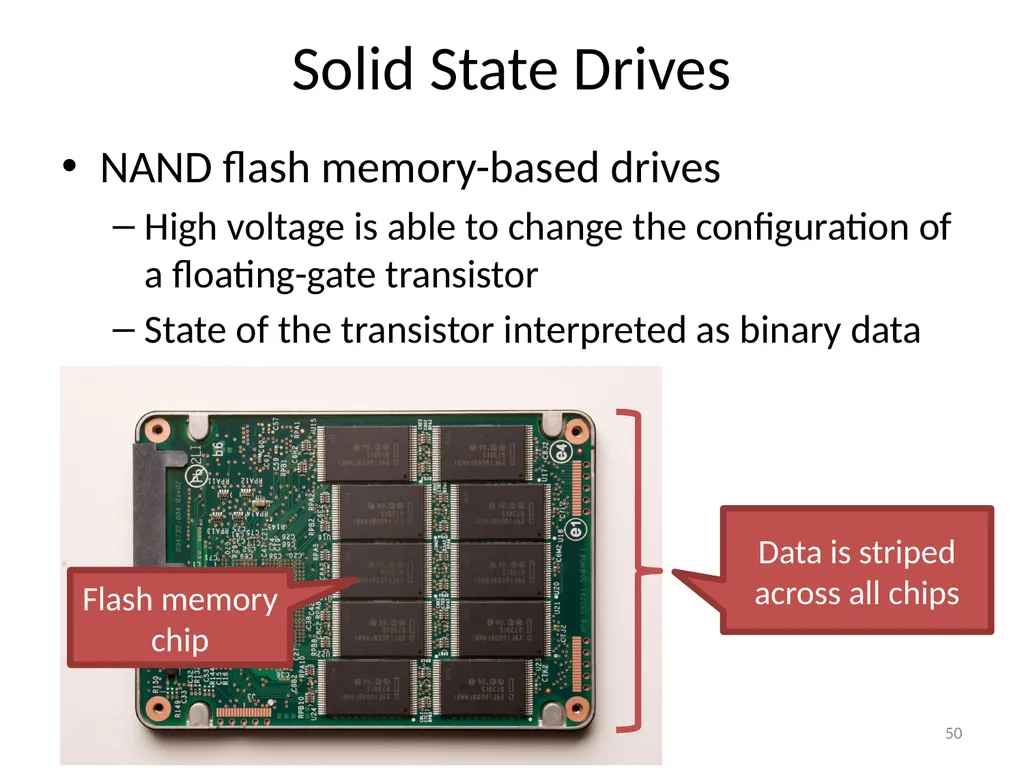
slide50. Solid State Drives NAND flash memory-based drives
High voltage is able to change the configuration of a floating-gate transistor
State of the transistor interpreted as binary data 50 Flash memory chip Data is striped across all chips<br>
slide51. Advantages of SSDs More resilient against physical damage
No sensitive read head or moving parts
Immune to changes in temperature
Greatly reduced power consumption
No mechanical, moving parts
Much faster than hard drives
>500 MB/s vs ~200 MB/s for hard drives
No penalty for random access
Each flash cell can be addressed directly
No need to rotate or seek
Extremely high throughput
Although each flash chip is slow, they are RAIDed 51<br>
slide52. 52<br>
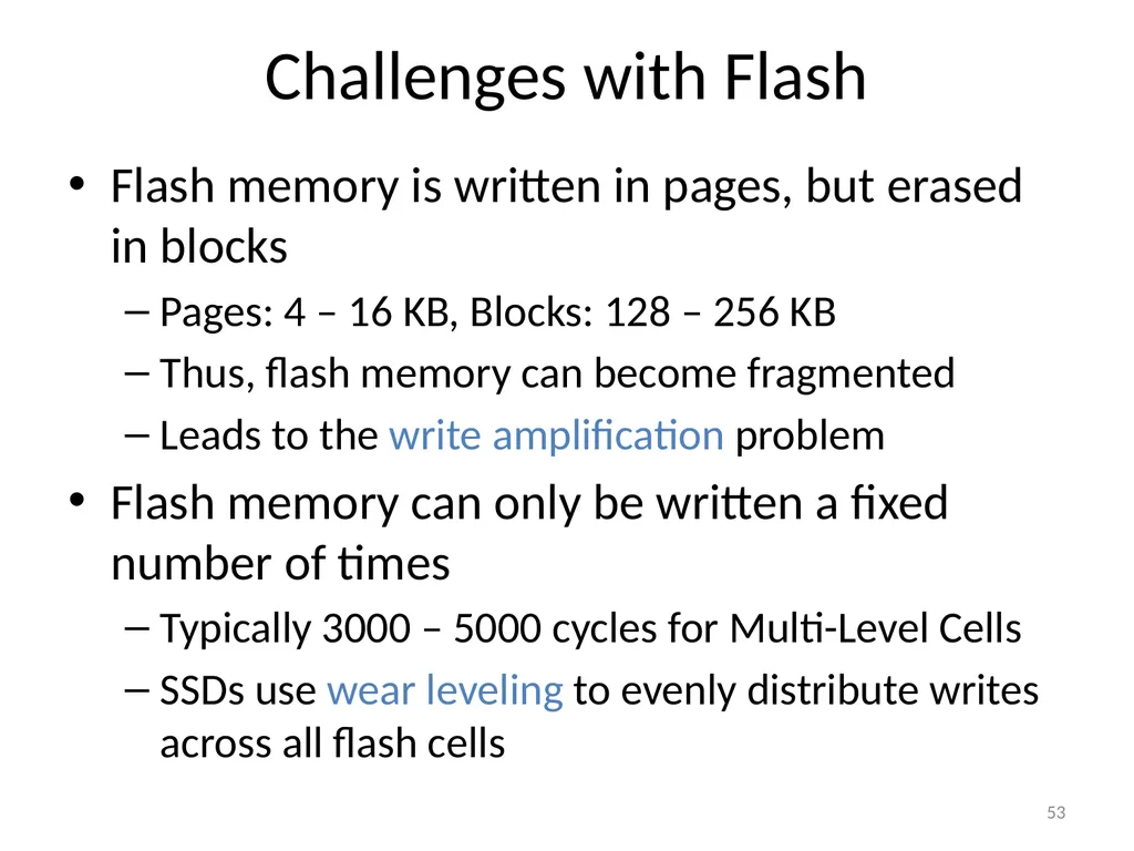
slide53. Challenges with Flash Flash memory is written in pages, but erased in blocks
Pages: 4 – 16 KB, Blocks: 128 – 256 KB
Thus, flash memory can become fragmented
Leads to the write amplification problem
Flash memory can only be written a fixed number of times
Typically 3000 – 5000 cycles for Multi-Level Cells
SSDs use wear leveling to evenly distribute writes across all flash cells 53<br>
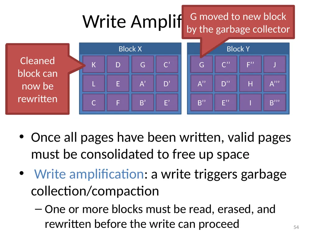
slide54. Write Amplification Once all pages have been written, valid pages must be consolidated to free up space
Write amplification: a write triggers garbage collection/compaction
One or more blocks must be read, erased, and rewritten before the write can proceed 54 A B C D E F G A’ B’ C’ D’ E’ F’ D’’ E’’ F’’ H I J A’’’ B’’’ A’’ B’’ C’’ Stale pages cannot be overwritten or erased individually G K L G moved to new block by the garbage collector Cleaned block can now be rewritten<br>
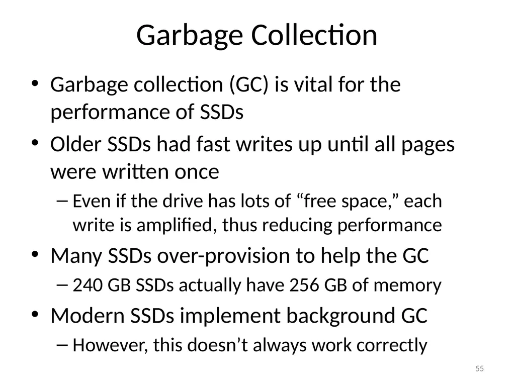
slide55. Garbage Collection Garbage collection (GC) is vital for the performance of SSDs
Older SSDs had fast writes up until all pages were written once
Even if the drive has lots of “free space,” each write is amplified, thus reducing performance
Many SSDs over-provision to help the GC
240 GB SSDs actually have 256 GB of memory
Modern SSDs implement background GC
However, this doesn’t always work correctly 55<br>
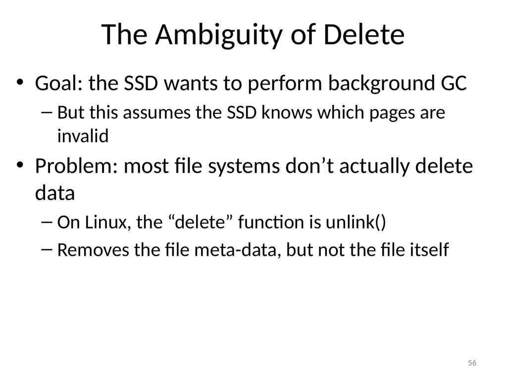
slide56. The Ambiguity of Delete Goal: the SSD wants to perform background GC
But this assumes the SSD knows which pages are invalid
Problem: most file systems don’t actually delete data
On Linux, the “delete” function is unlink()
Removes the file meta-data, but not the file itself 56<br>
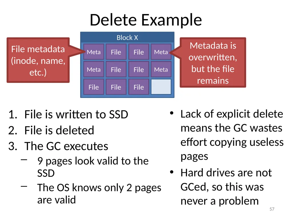
slide57. Delete Example File is written to SSD
File is deleted
The GC executes
9 pages look valid to the SSD
The OS knows only 2 pages are valid 57 Meta Meta File File File File File File File Meta Meta File metadata (inode, name, etc.) Metadata is overwritten, but the file remains Lack of explicit delete means the GC wastes effort copying useless pages
Hard drives are not GCed, so this was never a problem<br>
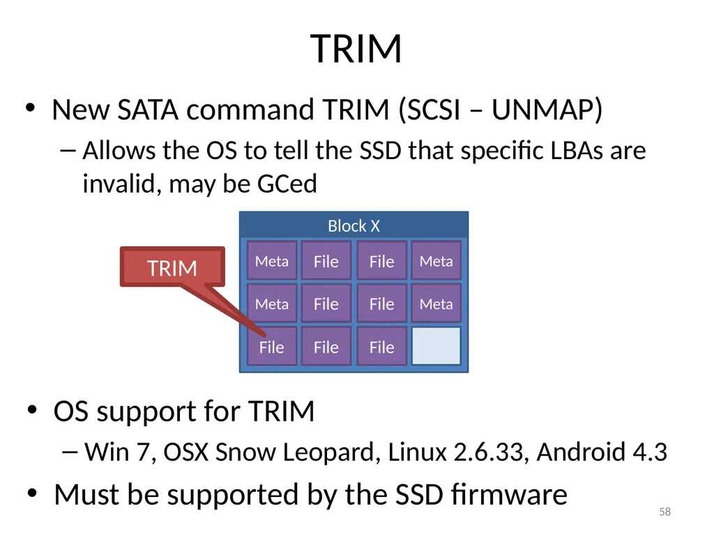
slide58. TRIM New SATA command TRIM (SCSI – UNMAP)
Allows the OS to tell the SSD that specific LBAs are invalid, may be GCed 58 OS support for TRIM
Win 7, OSX Snow Leopard, Linux 2.6.33, Android 4.3
Must be supported by the SSD firmware Meta Meta File File File File File File File Meta Meta TRIM<br>
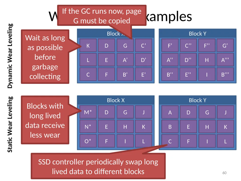
slide59. Wear Leveling Recall: each flash cell wears out after several thousand writes
SSDs use wear leveling to spread writes across all cells
Typical consumer SSDs should last ~5 years 59<br>
slide60. Wear Leveling Examples 60 A B C D E F G A’ B’ C’ D’ E’ F’ D’’ E’’ F’’ H I G’ A’’’ B’’’ A’’ B’’ C’’ K L Wait as long as possible before garbage collecting M N O M’ N’ O’ M’’ N’’ O’’ M’’’ N’’’ O’’’ M* N* O* M* N* SSD controller periodically swap long lived data to different blocks Blocks with long lived data receive less wear If the GC runs now, page G must be copied O* Dynamic Wear Leveling Static Wear Leveling<br>
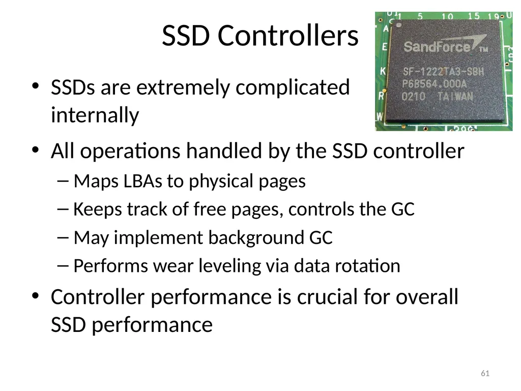
slide61. SSD Controllers All operations handled by the SSD controller
Maps LBAs to physical pages
Keeps track of free pages, controls the GC
May implement background GC
Performs wear leveling via data rotation
Controller performance is crucial for overall SSD performance 61 SSDs are extremely complicated internally<br>
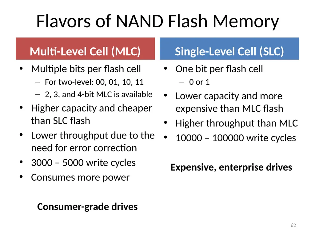
slide62. Flavors of NAND Flash Memory Multi-Level Cell (MLC) One bit per flash cell
0 or 1
Lower capacity and more expensive than MLC flash
Higher throughput than MLC
10000 – 100000 write cycles

Expensive, enterprise drives Single-Level Cell (SLC) Multiple bits per flash cell
For two-level: 00, 01, 10, 11
2, 3, and 4-bit MLC is available
Higher capacity and cheaper than SLC flash
Lower throughput due to the need for error correction
3000 – 5000 write cycles
Consumes more power

Consumer-grade drives 62<br>