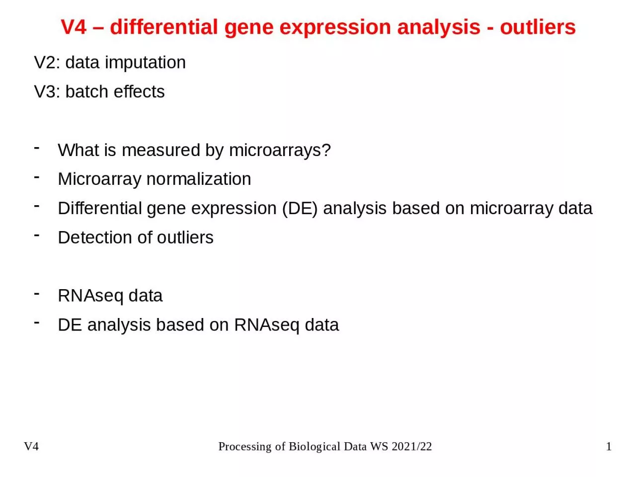
V4 – differential gene expression analysis - outliers - PowerPoint Presentation

1. V4 – differential gene expression analysis - outliersV2: data imputation V3: batch effectsWhat is measured by microarrays?Microarray normalizationDifferential gene expression (DE) analysis based on microarray dataDetection of outliersRNAseq dataDE analysis based on RNAseq data1V4Processing of Biological Data WS 2021/22

2. What is measured by microarrays?Microarrays are a collection of DNA probes that are bound in defined positions to a solid surface, such as a glass slide. The probes are generally oligonucleotides that are ‘ink-jet printed’ onto slides (Agilent) or synthesised in situ (Affymetrix). Labelled single-stranded DNA or antisense RNA fragments from a sample are hybridised to the DNA microarray. The amount of hybridisation detected for a specific probe is proportional to the number of nucleic acid fragments in the sample.2V4Processing of Biological Data WS 2021/22http://www.ebi.ac.uk/training/online/course/functional-genomics-ii-common-technologies-and-data-analysis-methods/microarrays

3. 2-color microarrays3V4Processing of Biological Data WS 2021/22http://www.ebi.ac.uk/training/online/course/functional-genomics-ii-common-technologies-and-data-analysis-methods/microarrayswww.sciencedirect.comIn 2-colour microarrays, 2 biological samples are labelled with different fluorescent dyes, usually Cyanine 3 (Cy3) and Cyanine 5 (Cy5). Equal amounts of labelled cDNA are then simultaneously hybridised to the same microarray chip. Then, the fluorescence measurements are made separately for each dye and represent the abundance of each gene in the test sample (Cy5) relative to the control sample (Cy3). 

4. MicroArray Quality Control (MAQC) project (2006)4V4Processing of Biological Data WS 2021/22Nature Biotechnology 24, 1151–1161(2006)MAQC project: community-wide effort that was initiated and led by FDA scientists involving 137 participants from 51 organizations. In this project, gene expression levels were measured - from 2 high-quality, distinct RNA samples (Universal Human Reference RNA (UHRR) from Stratagene and a Human Brain Reference RNA (HBRR) from Ambion) - in 4 titration pools (Sample A, 100% UHRR; Sample B, 100% HBRR; Sample C, 75% UHRR:25% HBRR; and Sample D, 25% UHRR:75% HBRR.)- on 7 microarray platforms (Applied Biosystems (ABI); Affymetrix (AFX); Agilent Technologies (AGL for two-color and AG1 for one-color); GE Healthcare (GEH); Illumina (ILM) and Eppendorf (EPP))- and 3 alternative expression methodologies (TaqMan Gene Expression Assays; StaRT-PCR from Gene Express (GEX) and QuantiGene assays from Panomics (QGN)). Each microarray platform was deployed at 3 independent test sites and 5 replicates were assayed at each site. Aim of this study: find out how reproducable MA experiments are.

5. MicroArray Quality Control (MAQC) project5V4Processing of Biological Data WS 2021/22Nature Biotechnology 24, 1151–1161(2006)The coefficient of variation (CV) relates standard deviation to mean.Shown here is CV of the signal (not log transformed) between the intrasite replicates (n ≤ 5) for genes that were detected in at least 3 replicates of the same sample type within a test site. Most of the one-color microarray platforms and test sites demonstrated similar replicate CV median values of 5–15%.

6. MicroArray Quality Control (MAQC) project6V4Processing of Biological Data WS 2021/22Nature Biotechnology 24, 1151–1161(2006)Concordance of genes identified as differentially expressed for pairs of test sites, labeled as X and Y.light-colored square: high percent overlap between the gene lists at both test sites. dark-colored square: low percent overlapFor all but the NCI test sites, the gene list overlap is at least 60% for each test site comparison (both directions) with many site pairings achieving 80% or more between platforms and 90% within platforms.

7. Analysis of microarray data: workflow7V4Processing of Biological Data WS 2021/22http://www.ebi.ac.uk/training/online/course/functional-genomics-ii-common-technologies-and-data-analysis-methods/microarraysMicroarrays can be used in many types of experiments including - genotyping, - epigenetics, - translation profiling and - gene expression profiling.Gene expression profiling is by far the most common use of microarray technology. Both one and two colour microarrays can be used for this type of experiment.

8. Quality control (QC) is done on the raw data8V4Processing of Biological Data WS 2021/22http://www.ebi.ac.uk/training/online/course/functional-genomics-ii-common-technologies-and-data-analysis-methods/microarraysQC of microarray data begins with the visual inspection of the scanned microarray images to make sure that there are no obvious splotches, scratches or blank areas.Data analysis software packages produce different sorts of diagnostic plots, e.g. of background signal, average intensity values and percentage of genes above background to help identify problematic arrays, reporters or samples.Box plot PCA Density plotexpression expression

9. Normalisation9V4Processing of Biological Data WS 2021/22http://www.ebi.ac.uk/training/online/course/functional-genomics-ii-common-technologies-and-data-analysis-methods/microarraysNormalisation is used to control for technical variation between assays, while preserving the biological variation. There are many ways to normalise the data. The methods used depend on:- the type of array;- the design of the experiment;- assumptions made about the data;- and the package being used to analyse the data.For the Expression Atlas at EBI, Affymetrix microarray data is normalised using the 'Robust Multi-Array Average' (RMA) method within the 'oligo' package (which is based on quantile normalization).Agilent microarray data is normalised using the 'limma' package: 'quantile normalisation' for one-colour microarray data; 'Loess normalisation' for two colour microarray data.

10. Differential expression analysis: Fold change10V4Processing of Biological Data WS 2021/22Cui & Churchill, Genome Biol. 2003; 4(4): 210. The simplest method to identify DE genes is to evaluate the log ratio between two conditions (or the average of ratios when there are replicates) and consider all genes that differ by more than an arbitrary cut-off value to be differentially expressed. E.g. the cut-off value chosen could be chosen as a two-fold difference. Then, all genes are taken to be differentially expressed if the expression under one condition is over two-fold greater or less than that under the other condition. This test, sometimes called 'fold' change, is not a statistical test.→ there is no associated value that can indicate the level of confidence in the designation of genes as differentially expressed or not differentially expressed.

11. Standard error of the mean11V4Processing of Biological Data WS 2021/22The standard deviation σ gives the „standard“ deviation of all measurements.Often we are more interested in the standard deviation of the average.This is denoted by the standard error of the mean (SEM):Whenever we use a random sample as estimate for a population, there is a good chance that our estimate will contain an error.SEM provides an estimate for this error.Typically, we actually need to compute SEM for the difference of the means of two random samples  2-sample t-test.

12. t-tests12V4Processing of Biological Data WS 2021/22t-value: by how many standard errors does a difference differ from 0?There are 3 different types of t-tests:Unpaired t-test Paired t-test1-sample t-test 

13. t distribution13V4Processing of Biological Data WS 2021/22The form of the t-distribution is very similar to a standard normal distribution – at least for large random samples.For small random samples, the t-distribution is flatter than a normal distribution.Therefore, the t-distribution needs another parameter that adjusts its variance (and thus its shape). This parameter is called the degrees-of-freedom; abbreviated as df.https://matheguru.com/stochastik/t-test.html

14. 1-sample t-test14V4Processing of Biological Data WS 2021/22A t-test is a parametric statistical hypothesis test that can be used when the population conforms to a normal distribution. A frequently used t-test is the one-sample location t-test that tests whether the mean of a normally distributed population has a particular value 0,where : sample mean,  : standard deviation of the sample, n : sample size. The critical value of the t-statistic t0 is tabulated in t-distribution tables. The hypothesis (H0) is that the population mean equals 0.If the p-value is below a threshold, e.g. 0.05, the null hypothesis is rejected.   

15. 2-sample t-test15V4Processing of Biological Data WS 2021/22The 2-sample t-tests measures Assumptions: both random samples have close to normal distribution and they have the same standard deviation. estimatedvariance of X1estimatedvariance of X2Degrees offreedomCorrection of SEMhttps://matheguru.com/stochastik/t-test.htmlIf 2 random variables X and Y are independent, the variance of their sum is the sum of the individual variancesV(X+Y)=V(X)+V(Y)

16. Limma Package: Volcano plot16V4Processing of Biological Data WS 2021/22Rapaport et al. (2013) Genome Biol. 14: R95Cui & Churchill, Genome Biol. 2003; 4(4): 210The 'volcano plot' is an easy-to-interpret graph that summarizes both fold-change and t-test criteria. It is a scatter-plot of the negative log10-transformed p-values from the gene-specific t test against the log2 fold change. Genes with statistically significant differential expression according to the gene-specific t test will lie above a horizontal threshold line. Genes with large fold-change values will lie outside a pair of vertical threshold lines. The significant genes identified by the S, B, and regularized t tests will tend to be located in the upper left or upper right parts of the plot.

17. Detection of Outlier Samples/Genes17V4Processing of Biological Data WS 2021/22Outlier : an observation that deviates “too much” from other observations. Detecting outliers might be important either because the outlier observations are of interest themselves or because they might contaminate the downstream statistical analysis. One common reason for outliers is mislabeling, where accidently a sample of one class might be falsely assigned to another one. An outlier might also be a gene with abnormal expression values in one or more samples from the same class. In the case of cancer, this may reflect that this patient or his/her disease is a special case.

18. Grubbs test18V4Processing of Biological Data WS 2021/22Grubbs’ test can be used to test the presence of one outlier and can be used with data that is normally distributed (except for the outlier) and has at least 7 elements (preferably more).One tests the null hypothesis that the data has no outliers vs. the alternative hypothesis that there is one outlier.If you suspect that the maximum (minimum) value in the data set may be an outlier you can use the test statisticThe critical value for the test iswhere tcrit is the critical value of the t distribution T(n−2) and the significance level is α/n. Thus the null hypothesis is rejected if G > Gcrit.http://www.real-statistics.com/students-t-distribution/identifying-outliers-using-t-distribution/grubbs-test/

19. GESD19V4Processing of Biological Data WS 2021/22GESD was developed to detect ≥1 outliers in a dataset assuming that the body of its data points comes from a normal distribution. First, GESD calculates the deviation between every point xi and the mean , normalized by the standard deviation.At each iteration, it then removes the point with the maximum deviation. This process is repeated until all outliers that fulfill the condition are identified where λ is the critical value calculated for all points using the percentage points of the t distribution.

20. GESD20V4Processing of Biological Data WS 2021/22GESD and its predecessor ESD will always mark at least one data point as outlier even when there are in fact no outliers present. Therefore, using GESD to detect outliers in microarray data must be accompanied with a threshold of outlier allowance where a certain amount of outliers are detected before marking a gene as an outlier. The GESD method is said to perform best for datasets with more than 25 points. Additionally, the algorithm requires the suspected amount of outliers as an input.

21. 8.4 Detect outliers with MADIn contrast to GESD, the MAD algorithm (Rousseeuw and Croux 1993) is not based on the variance or standard deviation and thus makes no particular assumption on the statistical distribution of the data. At first, the raw median is computed over all data points. From this, MAD obtains the median absolute deviation (MAD) of single data points Xi from the raw median as:b is a scaling constant. For normally distributed data, one uses b = 1.4826. As rejection criterion of outliers, one uses Suitable thresholds could be 3 (very conservative), 2.5 (moderately conservative) or 2 (poorly conservative).  V4Processing of Biological Data WS 2021/2221

22. 8.4 Detect outliers with MADConsider the data (1, 3, 4, 5, 6, 6, 7, 7, 8, 9, 100). It has a (raw) median value of 6. The absolute deviations from 6 are (5, 3, 2, 1, 0, 0, 1, 1, 2, 3, 94). Sorting this list into (0, 0, 1, 1, 1, 2, 2, 3, 3, 5, 94) shows that the deviations have a median value of 2. When scaled with b = 1.4826, the median absolute deviation (MAD) for this data is roughly 3. Possible outliers above a rejection threshold would need to differ from the median by 6 to 9 or more. For this example, only the extreme data point (100) deviates that much. V4Processing of Biological Data WS 2021/2222

23. Effect of 2 outliers on auto-correlation of a gene23V4Processing of Biological Data WS 2021/22Effect of 2 introduced outlier points on co-expression analysis of a gene with itself (4 datasets from TCGA for COAD; GBM; HCC, OV tumor).X-axis : magnitude of perturbations applied as multiples of standard deviations (SD).For the smallest sample (COAD), two 2SD outliers, reduce the auto- correlation to 0.75.Barghash et al., J Proteomics Bioinform 2016, 9:2

24. Simulated expression data sets24V4Processing of Biological Data WS 2021/22Different gray levels represent different classes. Outlier cases are in black. SDS1/2 (left) has two known outliers (black) and 3 known switched samples. SDS3/4 (right) contain 50 outliers each. SDS1-3 follow Gaussian distributions while SDS4 follows a Poisson distribution.Barghash et al., J Proteomics Bioinform 2016, 9:2

25. Clustering dendogram25V4Processing of Biological Data WS 2021/22Clustering dendrogram of dataset of simulated expression.Average Hierarchical Clustering based on Euclidean distances (AHC-ED) clustered SDS1 into 3 main classes grouping the outlier samples (50 and 100) in a separate class. All switched samples – marked by asterisks - were correctly clustered into their original classes.Barghash et al., J Proteomics Bioinform 2016, 9:2

26. Silhouette: validates clustering26V4Processing of Biological Data WS 2021/22Silhouette validation of the AHC-ED clustering of SDS1. The average distance of 0.36 indicates that AHC-ED succeeded in clustering SDS1.Silhouette coefficient:a(i) : average dissimilarity of i with all other data within the same clusterb(i) : lowest average dissimilarity of i to any other cluster, of which i is not a memberLarge s(i) means good clusteringBarghash et al., J Proteomics Bioinform 2016, 9:2

27. 27V4Processing of Biological Data WS 2021/22Bottom: If the two distributions have larger overlap (1 SD → 2 SD →3 SD), detecting outliers becomes considerably harder.# of detected synthetic outlier data points (out of 50)Top: In normally distributed data, GESD identified largest number (46/50) of synthetic outliers. Barghash et al., J Proteomics Bioinform 2016, 9:2

28. MA quality control28V4Processing of Biological Data WS 2021/22Kauffman, Huber (2010) Genomics 95, 138These authors compared four strategies of data analysis :- Strategy 1 No outlier removal- Strategy 2 Outlier removal guided by arrayQualityMetrics (outliers of boxplot)- Strategy 3 Removing random arrays (same number of arrays as in strategy 2)- Strategy 4 Array weights using the function arrayWeights from the limma Bioconductor package

29. Number of DE genes29V4Processing of Biological Data WS 2021/22Kauffman, Huber (2010) Genomics 95, 138Number of differentially expressed genes identified:on the whole dataset (white bars), after removing outliers identified by arrayQualityMetrics (black bars) and using weights obtained by arrayWeights from limma (grey bars).→ Many more DE genes identified after removing outlier genes.E-MEXP-170 has additional confounding effect of experiment date! This explains high # of DE genes.Data -> rma -> DE genes with moderated t-test in limma, FDR correction

30. Effect of Outlier removal on DE genes30V4Processing of Biological Data WS 2021/22Kauffman, Huber (2010) Genomics 95, 138Venn diagrams representing the number of DE genes identified by each method: all arrays, after removing outlier arrays, using array weights. (a) E-GEOD-3419, (b) E-GEOD-7258, (c) E-GEOD-10211, (d) E-MEXP-774, (e) E-MEXP-170.In (c), (d), (e) good overlap of outlier removal and weight method.

31. Effect of removing random genes on DE genes31V4Processing of Biological Data WS 2021/22Kauffman, Huber (2010) Genomics 95, 138Boxplots representing the number of DE genes in each experiment when removing arbitrary subsets of size K, the number of outlier arrays identified from the N samples. When N over K < 1000, all possible subsets were considered, otherwise 1000 subsets were sampled randomly.If the same number of random genes is removed, fewer DE genes are detected.

32. KEGG pathway enrichment analysis32V4Processing of Biological Data WS 2021/22Kauffman, Huber (2010) Genomics 95, 138gene set enrichment analysis :5 most enriched KEGG pathways among DE genes for experiments E-GEOD-3419 and E-GEOD-7258, with and without outlier removal. → The pathways are related to the biology studied in the experiments.→ Their enrichment is more significant after outlier removal.Does removal of outliers result in better biological sensitivity?

33. Results from other outlier detection methods33V4Processing of Biological Data WS 2021/22Kauffman, Huber (2010) Genomics 95, 138Comparison of different outlier detection methods: method implemented in arrayQualityMetrics (based on boxplots),generalized extreme studentized deviate (GESD), method of Hampel (it is based on the median absolute deviation (MAD)). The results of different methods overlap mostly -> robustness

34. DE analysis from RNAseq data34V4Processing of Biological Data WS 2021/22Rapaport et al. (2013) Genome Biol. 14: R95Cui & Churchill, Genome Biol. 2003; 4(4): 210Compared to microarrays, RNA-seq has the following advantages for DE analysis:- RNA-seq has a higher sensitivity for genes expressed either at low or very high level and higher dynamic range of expression levels over which transcripts can be detected (> 8000-fold range). It also has lower technical variation and higher levels of reproducibility. - RNA-seq is not limited by prior knowledge of the genome of the organism.  - RNA-seq detects transcriptional features, such as novel transcribed regions, alternative splicing and allele-specific expression at single base resolution. While Microarrays are subject to cross-hybridisation bias,RNA-seq may have a guanine-cytosine content bias and can suffer from mapping ambiguity for paralogous sequences.

35. DE detection based on RNAseq dataRapaport et al. (2013) Genome Biol. 14: R95If sequencing experiments are considered as random samplings of reads from a fixed pool of genes,then a natural representation of gene read counts is the Poisson distribution of the form where n : number of read counts  : expected number of reads from transcript fragments.An important property of the Poisson distribution is that variance AND mean are both equal to , However, in reality the variance of gene expression across multiple biological replicates is found to be larger than its mean expression values.  V4Processing of Biological Data WS 2021/2235

36. DE detection in RNAseq dataTo address this “over-dispersion problem”, methods such as edgeR and DESeq use the related negative binomial distribution (NB) where variance and mean μ is are related to each other bywhere  is the “dispersion factor”.Different software packages (e.g. edgeR and DESeq, both by the Huber group) use different ways to estimate this dispersion factor.For more details on DESeq, see Bioinformatics III lecture #10.For the identification of differentially expressed genes, DESeq uses a test statistics similar to Fisher‘s exact test. However, DESeq was found to be „overly conservative“.This led to the development of DESeq2. V4Processing of Biological Data WS 2021/2236

37. Reference data: gold standard37V4Processing of Biological Data WS 2021/22Rapaport et al. (2013) Genome Biol. 14: R95Samples from group A : Strategene Universal Human Reference RNA (UHRR): total RNA from ten human cell lines. Samples from group B: Ambion’s Human Brain Reference RNA (HBRR). ERCC spike-in control : mixture of 92 synthetic polyadenylated oligonucleotides, 250 to 2,000 nucleotides long, which resemble human transcripts. The two ERCC mixtures in groups A and B contain different (known!) concentrations of 4 subgroups of the synthetic spike-ins.Then the log expression change is predefined and can be used to benchmark DE performance.

38. Performance for DE detection38V4Processing of Biological Data WS 2021/22Rapaport et al. (2013) Genome Biol. 14: R95ERCC control oligonucleotides were divided into four groups with different mixing ratios between samples A and B (1:1, 4:1, 1:2 and 2:3). In this ROC analysis the 1:1 mix are the set of undifferentiated controls (true negatives) and all others are differentiated (true positives). AUC = area under the curve.All methods performed reasonably well in detecting the truly differentiated spike-in sequences with an average area under the curve (AUC) of 0.78

39. Performance for DE detection39V4Processing of Biological Data WS 2021/22Rapaport et al. (2013) Genome Biol. 14: R95Differential expression analysis using qRT-PCR validated gene setof about 1000 genes from the MACQ project (slides 4-6). ROC analysis was performed using a qRT-PCR log2 expression change threshold of 0.5.If the change is >0.5, the gene is DE, otherwise not. The results are quite comparable.DESeq and edgeR have slightly higher detection accuracy.

40. Performance for DE detection40V4Processing of Biological Data WS 2021/22Rapaport et al. (2013) Genome Biol. 14: R95If one measures AUC at increasing cutoff values of qRT-PCR expression changes, this should define sets of DE genes at increasing stringency. Now, there is a significant performance advantage for negative binomial and Poisson-based approaches with consistent AUC values close to 0.9 or higher. On the other hand, Cuffdiff and limma methods display decreasing AUC values indicating reduced discrimination power at higher expression change log values.

41. Current situation: detecting DE genes from RNAseq data41V4Processing of Biological Data WS 2021/22Normalization of RNA-seq read counts is an essential procedure that corrects for non-biological variation of samples due to library preparation, sequencing readdepth, gene length, mapping bias and other technical issues. There are many normalization methods to correct for technical variations and biases:Some methods correct for read depth and transcript length: RPKM (Reads Per Kilobase per Million mapped reads) – used by package DEGSeqHere, 103 normalizes for gene length and 106 for sequencing depth factor.E.g. you have sequenced one library with 5 M reads. Among them, total 4 M matched to the genome sequence and 5000 reads matched to a given gene with a length of 2000 bp.Li et al. BMC Genomics (2020) 21:75https://www.biostars.org/p/273537/

42. Current situation: detecting DE genes from RNAseq data42V4Processing of Biological Data WS 2021/22FPKM (Fragments Per Kilobase per Million mapped fragments) – CuffDiffFPKM is analogous to RPKM and used especially in paired-end RNA-seq experiments.Other methods use global scaling quantile normalization: TC (per-sample total counts), UQ (per-sample 75% upper quartile Q3), Med (per-sample Median Q2), or Q (full quantile) implemented in Aroma.light. DESeq/DESeq2 and edgeR use an imputed size factor to correct for read depth bias.RUV normalizes by the expression of control genes to remove unwanted technical variation across samples.Sailfish is an alignment-free abundance estimation using k-mers to index and count RNA-seq reads.Li et al. presented a method called UQ-pgQ2 (per-gene Q2 normalization following per-sample upper-quartile global scaling at 75 percentile) for correcting library depths and scaling the reads of each gene into the similar levels across conditions.

43. Comparison of different methods43V4Processing of Biological Data WS 2021/22Other earlier studies were left out.Li et al. BMC Genomics (2020) 21:75

44. Outlier detection for RNA-seq data: Outrider44V4Processing of Biological Data WS 2021/22Normalized RNA-seq read counts plotted against their rank (A and C) and quantile-quantile plots of observed p values against expected p values with 95% confidence bands (B and D); outliers are shown in red (FDR < 0.05). Shown are data for TRIM33 with no detected expression outlier (A and B) and data for SLC39A4 with two expression outliers (C and D).Brechtmann … Gagneur, Am J Hum Genet. (2018) 103, 907-917.Based on synthetic data, an autoencoder is entrained to detect outlier data points.Outlier detection is equally important when processing RNA-seq data.

45. Convolution of bulk sequencing data45V4Processing of Biological Data WS 2021/22Genotype-tissue expression (GTEx) project:over 10,000 bulk RNA-seq samples representing 53 different tissues from 30 organs obtained from 635 genotyped individuals.The aim is to link the influence of genetic variants on gene expression levels through quantitative trait loci analysis (eQTL).Problem: data set does not account for cellular heterogeneity (i.e., different cell types within a tissue and the relative proportions of each cell type across samples of the same tissue)Possible solution: deconvolute data into separate cell types.Donovan et al. (2020) Nature Commun. 11:955

46. Convolution of bulk sequencing data46V4Processing of Biological Data WS 2021/22In a proof-of-concept analysis, the cellular estimates of 2 GTEx tissues (liver and skin) were deconvoluted using both mouse and human signature genes obtained from scRNA-seq. We then performed cellular deconvolution of the 28 GTEx tissues from 14 organs using CIBERSORT and characterized both the heterogeneity in cellular composition between tissues and the heterogeneity in relative distributions of cell populations between RNA-seq samples from a given tissue. Finally, we used the cell type composition estimates as interaction terms for eQTL analyses to determine if we could detect cell-type-associated genetic associations.Donovan et al. (2020) Nature Commun. 11:955

47. CIBERSORT47V4Processing of Biological Data WS 2021/22Deconvolution of gene expression profiles (GEP) can be represented by M = f × B, provided that B contains more marker genes than cell types (i.e., the system is overdetermined).M : mRNA mixtureB : GEP signature matrixf : vector consisting of the unknown fractions of each cell type in the mixture Previous groups have applied linear least squares regression (LLSR) and more recently, non-negative least squares regression (NNLS) and quadratic programming (QP) to solve for f.Cibersort uses ν-support vector regression (details are not important here).Newman et al. Nature Methods 12, 453–457 (2015)

48. Convolution of bulk sequencing data48V4Processing of Biological Data WS 2021/22Bar plots showing the fraction of cell types estimated in the 175 GTEx liver RNA-seq samples deconvoluted using c gene expression profiles from high-resolution human liver scRNA-seq, or d from low-resolution mouse liver scRNA-seq, ore GTEx estimates generated by collapsing high-resolution human cell types within each of the seven distinct cell classes.Hepatocyte estimates from mouse liver were positively and highly correlated with the human high-resolution hepatocyte 0 population estimate (r = 0.71, p-value = 5.4 × 10−28).Donovan et al. (2020) Nature Commun. 11:955

49. Summary49V4Processing of Biological Data WS 2021/22Removing outlier data sets from the input data is essential for the downstream analysis (unless these outliers are of particular interest -> personalized medicine).Analysis tools: box-plots, PCA, density plots, clusteringSome outlier methods (GESD) are based on variants of the t-test.MAD and boxplots are other simple methods.Normalization of RNA-seq data: many different strategies exist.Single-cell data based deconvolution of bulk sequencing data can help in increasing the insight that can be obtained from existing bulk data.

50. Additional slides (not used)50V4Processing of Biological Data WS 2021/22

51. CIBERSORT uses nu–support vector regression (ν-SVR).51V4Processing of Biological Data WS 2021/22ν-SVR is an instance of support vector machine (SVM), a class of optimization methods for binary classification problems, in which a hyperplane is discovered that maximally separates both classes. The support vectors are a subset of the input data that determine hyperplane boundaries. Unlike standard SVM, SVR discovers a hyperplane that fits as many data points as possible (given its objective function) within a constant distance, ɛ, thus performing a regression. All data points within ɛ (termed the ‘ɛ-tube’) are ignored, whereas all data points lying outside of the ɛ-tube are evaluated according to a linear ɛ-insensitive loss function. These outlier data points, referred to as ‘support vectors’, define the boundaries of the ɛ-tube and are sufficient to completely specify the linear regression function. In this way, support vectors can provide a sparse solution to the regression in which overfitting is minimized (a type of feature selection). Notably, support vectors represent genes selected from the signature matrix in this work.Newman et al. Nature Methods 12, 453–457 (2015)

52. CIBERSORT52V4Processing of Biological Data WS 2021/22A simple 2D dataset analyzed with linear ν-SVR, with results shown for two values of ν (note that both panels show the same data points). As linear SVR identifies a hyperplane (which, in this 2D example, is a line) that fits as many data points as possible (given its objective function) within a constant distance, ɛ (open circles). Data points lying outside of this ‘ɛ-tube’ are termed ‘support vectors’ (red circles), and are penalized according to their distance from the ɛ-tube by linear slack variables (ξi). Newman et al. Nature Methods 12, 453–457 (2015)Importantly, the support vectors alone are sufficient to completely specify the linear function, and provide a sparse solution to the regression that reduces the chance of overfitting. In ν-SVR, the ν parameter determines both the lower bound of support vectors and upper bound of training errors. As such, higher values of ν result in a smaller ɛ-tube and a greater number of support vectors (right panel). For CIBERSORT, the support vectors represent genes selected from the signature matrix for analysis of a given mixture sample, and the orientation of the regression hyperplane determines the estimated cell type proportions in the mixture.

53. CIBERSORT53V4Processing of Biological Data WS 2021/22CIBERSORT requires an input matrix of reference gene expression signatures, collectively used to estimate the relative proportions of each cell type of interest. To deconvolve the mixture, we employ a novel application of linear support vector regression (SVR), a machine learning approach highly robust with respect to noise. Unlike previous methods, SVR performs a feature selection, in which genes from the signature matrix are adaptively selected to deconvolve a given mixture. An empirically defined global P value for the deconvolution is then determined.Newman et al. Nature Methods 12, 453–457 (2015)

54. Extraction of features54V4Processing of Biological Data WS 2021/22http://www.ebi.ac.uk/training/online/course/functional-genomics-ii-common-technologies-and-data-analysis-methods/microarraysFeature extraction is the process of converting the scanned image of the microarray into quantifiable values and annotating it with the gene IDs, sample names and other useful information This process is often performed using the software provided by the microarray manufacturer. ManufacturerTypical raw data formatHow to open / Analysis software examplesAffymetrix .CEL (binary)R packages (affy, limma, oligo…)Agilentfeature extraction file (tab-delimited text file per hybridisation)Spreadsheet software (Excel, OpenOffice, etc.)GenePix (scanner).gpr (tab-delimited text file per hybridisation)Spreadsheet software (Excel, OpenOffice, etc.)Illumina.idat (binary)R packages (e.g. illuminaio)txt (tab-delimited text matrix for all samples)Spreadsheet software (Excel, OpenOffice, etc.)NimblegenNimbleScan, .pair (tab-delimited text matrix for all samples)Spreadsheet software (Excel, OpenOffice, etc.) Common microarray raw data file types.